聊聊 神經網路模型 預訓練生成超引數實現

概述

在上一篇部落格中，已經闡述了預訓練過程中，神經網路中超引數的計算邏輯，本文，從程式實現的角度，將數學計算轉換為程式程式碼，最終生成超引數檔案；並將替換 聊聊 神經網路模型 範例程式——數位的推理預測 中已訓練好的超引數檔案，推理預測數位，最終比對下兩者的精確度。

神經網路層實現

首先，根據神經網路各個層的計算邏輯用程式實現相關的計算，主要是：前向傳播計算、反向傳播計算、損失計算、精確度計算等，並提供儲存超引數到檔案中。

# coding: utf-8
import sys, os
sys.path.append(os.pardir)  # 為了匯入父目錄的檔案而進行的設定
from DeepLearn_Base.common.functions import *
from DeepLearn_Base.common.gradient import numerical_gradient
import pickle

# 三層神經網路處理類(兩層隱藏層+1層輸出層)
class ThreeLayerNet:

    # input_size:輸入層神經元數量，灰度影象的三維表示: 1 * 28 * 28 = 784
    # output_size: 輸出層神經元數量，10，表示10個數位
    # hidden_size：第一層隱藏層神經元數量，50
    # second_hidden_size：第二層隱藏層神經元數量，100
    # weight_init_std：權重初始化
    def __init__(self, input_size, hidden_size, output_size, second_hidden_size, weight_init_std=0.01):
        # 初始化權重
        self.params = {}
        self.params['W1'] = weight_init_std * np.random.randn(input_size, hidden_size)
        self.params['b1'] = np.zeros(hidden_size)
        self.params['W2'] = weight_init_std * np.random.randn(hidden_size, second_hidden_size)
        self.params['b2'] = np.zeros(second_hidden_size)
        self.params['W3'] = weight_init_std * np.random.randn(second_hidden_size, output_size)
        self.params['b3'] = np.zeros(output_size)

    # 執行預測
    def predict(self, x):
        W1, W2, W3 = self.params['W1'], self.params['W2'], self.params['W3']
        b1, b2, b3 = self.params['b1'], self.params['b2'], self.params['b3']
    
        # 隱藏層第一層
        a1 = np.dot(x, W1) + b1
        z1 = sigmoid(a1)

        # 隱藏層第二層
        a2 = np.dot(z1, W2) + b2
        z2 = sigmoid(a2)
        
        # 輸出層
        a3 = np.dot(z2, W3) + b3
        y = softmax(a3)
        
        return y
        
    # x:輸入資料, t:監督資料
    def loss(self, x, t):
        y = self.predict(x)
        
        return cross_entropy_error(y, t)
    
    # 精確度計算
    def accuracy(self, x, t):
        y = self.predict(x)
        y = np.argmax(y, axis=1)
        t = np.argmax(t, axis=1)
        
        accuracy = np.sum(y == t) / float(x.shape[0])
        return accuracy
        
    # 梯度計算
    def gradient(self, x, t):
        W1, W2, W3 = self.params['W1'], self.params['W2'], self.params['W3']
        b1, b2, b3 = self.params['b1'], self.params['b2'], self.params['b3']
        grads = {}
        
        batch_num = x.shape[0]
        
        # forward
        # 隱藏層第一層
        a1 = np.dot(x, W1) + b1
        z1 = sigmoid(a1)

        # 隱藏層第二層
        a2 = np.dot(z1, W2) + b2
        z2 = sigmoid(a2)
        
        # 輸出層
        a3 = np.dot(z2, W3) + b3
        y = softmax(a3)
        
        # backward
        # 兩層隱藏層計算梯度
        # 輸出層梯度: Loss與輸出的導數，分類場景下，等於預測值-真實值
        # 權重梯度: 隱藏層輸出的轉置 * 損失函數梯度
        dy = (y - t) / batch_num
        grads['W3'] = np.dot(z2.T, dy)
        grads['b3'] = np.sum(dy, axis=0)
        
        # 反向傳播到隱藏層
        # 隱藏層梯度:Loss與輸出的導數 * 輸出層權重的轉置
        da2 = np.dot(dy, W3.T)
        dz2 = sigmoid_grad(a2) * da2
        grads['W2'] = np.dot(z1.T, dz2)
        grads['b2'] = np.sum(dz2, axis=0)

        da1 = np.dot(da2, W2.T)
        dz1 = sigmoid_grad(a1) * da1
        grads['W1'] = np.dot(x.T, dz1)
        grads['b1'] = np.sum(dz1, axis=0)

        return grads
    
    # 儲存引數到檔案
    def save_params(self, file_name="params.pkl"):
        params = {}
        for key, val in self.params.items():
            params[key] = val
        with open(file_name, 'wb') as f:
            pickle.dump(params, f)

預訓練實現

讀取MNIST訓練資料集，總共有60000個。每次從60000個訓練資料中隨機取出100個資料 (影象資料和正確解標籤資料)。然後，對這個包含100筆資料的批資料求梯度，使用隨機梯度下降法(SGD)更新引數。這裡，梯度法的更新次數(迴圈的次數)為10000。每更新一次，都對訓練資料計算損失函數的值，並把該值新增到陣列中。

# coding: utf-8
import sys, os
sys.path.append(os.pardir)  # 為了匯入父目錄的檔案而進行的設定
import numpy as np
import matplotlib.pyplot as plt
from DeepLearn_Base.dataset.mnist import load_mnist
from three_layer_net import ThreeLayerNet

# 讀入資料
# x_train.sharp 60000 * 784
# t_train.sharp 60000 * 10
(x_train, t_train), (x_test, t_test) = load_mnist(normalize=True, one_hot_label=True)

network = ThreeLayerNet(input_size=784, hidden_size=50, second_hidden_size=100, output_size=10)

iters_num = 10000  # 適當設定迴圈的次數
# 訓練集大小 60000
train_size = x_train.shape[0]
batch_size = 100
learning_rate = 0.1

train_loss_list = []
train_acc_list = []
test_acc_list = []

# 每批次迭代數量：600
iter_per_epoch = max(train_size / batch_size, 1)

for i in range(iters_num):
    # 從訓練集中選取100個為一批次進行訓練
    batch_mask = np.random.choice(train_size, batch_size)
    x_batch = x_train[batch_mask]
    t_batch = t_train[batch_mask]
    
    # 更新超引數梯度
    grad = network.gradient(x_batch, t_batch)
    
    # 更新超引數W,b
	# 基於SGD演演算法更新梯度，上面是隨機選擇的批資料處理，因此更新時，也是隨即更新梯度
    for key in ('W1', 'b1', 'W2', 'b2', 'W3', 'b3'):
        network.params[key] -= learning_rate * grad[key]
    
    loss = network.loss(x_batch, t_batch)
    train_loss_list.append(loss)
    
    if i % iter_per_epoch == 0:
        train_acc = network.accuracy(x_train, t_train)
        test_acc = network.accuracy(x_test, t_test)
        train_acc_list.append(train_acc)
        test_acc_list.append(test_acc)
        print("train acc, test acc | " + str(train_acc) + ", " + str(test_acc))

# 繪製圖形
markers = {'train': 'o', 'test': 's'}
x = np.arange(len(train_acc_list))
plt.plot(x, train_acc_list, label='train acc')
plt.plot(x, test_acc_list, label='test acc', linestyle='--')
plt.xlabel("epochs")
plt.ylabel("accuracy")
plt.ylim(0, 1.0)
plt.legend(loc='lower right')
plt.show()

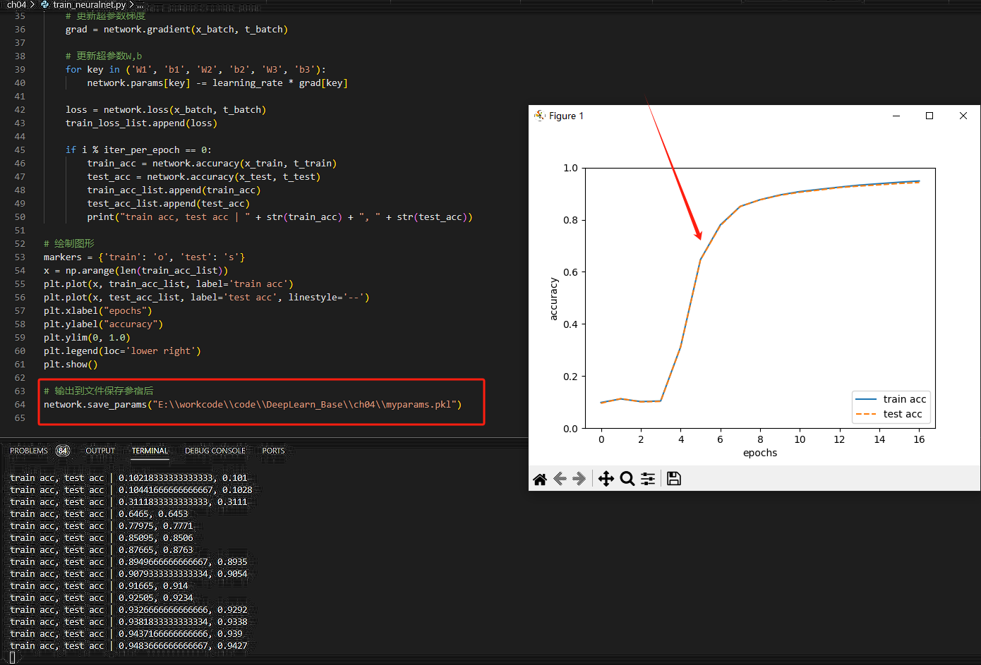
# 輸出到檔案儲存參宿後
network.save_params("E:\\workcode\\code\\DeepLearn_Base\\ch04\\myparams.pkl")

用影象來表示這個損失函數的值的推移，如圖所示；並儲存最終的超引數到pkl檔案。

應用自訓練超引數

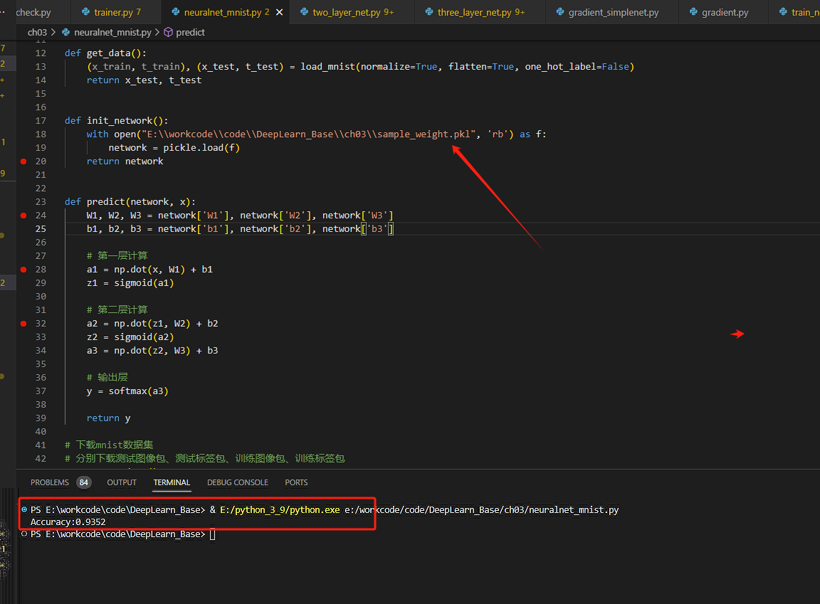
將之前用於預測影象文字中使用的超引數檔案替換為自己預訓練生成的pkl引數檔案，並執行程式碼，列印出精確度。
這是基於預設的超引數進行推理後的精確度：

替換超引數檔案，進行影象識別推理

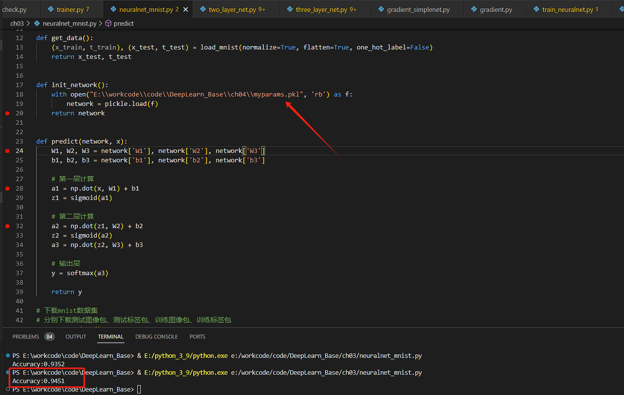
精確度上漲了0.01，因此選擇合適的梯度更新超引數，是保證推理精確度好壞的關鍵。