Pandas處理時間序列

Pandas最初是爲了處理金融模型而建立的,因此Pandas具有一些非常強大的日期,時間,帶時間索引數據的處理工具

本章將介紹的日期和時間數據主要包含三類:

時間戳:時間戳表示某個具體的時間點,例如2020年7月30日晚上10點41分
時間間隔與週期:時間間隔值兩個時間戳之間的時間長度,週期是具有相同長度,彼此不重疊的特殊的時間間隔
時間增量或持續時間:表示精確的時間間隔,例如一個程式的執行時間是24秒

下面下麪將介紹Pandas中的三種日期 / 時間數據型別的具體用法

Python的日期與時間工具

在講解Pandas的日期與時間工具之前首先講解下Python的原生的日期和時間工具(包括除了Pandas之外的第三方庫)

儘管Pandas提供的時間序列工具更加適合處理數據科學問題,但是瞭解Python標準庫和其他時間序列工具將會大有裨益

原生Python的日期與時間工具:datetime與dateutil

Python原生的基本的日期和時間功能都在datetime標準庫的datetime模組中,我們可以和第三方庫dateutil結合就可以快速實現許多處理日期和時間的功能

建立日期

我們可以使用datetime模組中的datetime物件建立一個日期

from datetime import datetime


datetime_1=datetime(year=2020,month=7,day=30)
print(datetime_1)
>>>
2020-07-30 00:00:00

或者我們可以使用dateutil庫的parser模組來對字串格式的日期進行解析(但是隻能用英美日期格式),使用parse函數解析將會得到一個datetime物件

from dateutil import parser

datetime_1=parser.parse('30th of July, 2020')
datetime_2=parser.parse('July 30th,2020')
print(datetime_1)
print(datetime_2)
>>>
2020-07-30 00:00:00
2020-07-30 00:00:00

指定輸出

一旦我們具有了一個datetime物件,我們就可以通過datetime物件的strftime方法來指定輸出的日期格式

from datetime import datetime
from dateutil import parser

datetime_1=parser.parse('30th of July, 2020')
print(datetime_1.strftime('%A'))
>>>
Thursday

這裏我們通過標準字串格式%A來指定輸出當前datetime物件的星期

實際上Python的datetime和dateutil物件模組在靈活性和易用性上的表現非常出色,但是就像前面不斷提起的,使用Python原生的datetime物件處理時間資訊在面對大型數據集的時候效能沒有Numpy中經過編碼的日期型別陣列效能好

Numpy的日期與時間工具:datetime64型別

Numpy團隊爲了解決Python原生陣列的效能弱點開發了自己的時間序列型別,datetime64型別將日期編碼爲64位元整數,這樣能夠讓日期陣列非常緊湊,從而節省記憶體.

Numpy建立日期陣列

我們在建立Numpy的日期陣列時,只需要指定數據型別爲np.datetime64即可建立日期陣列

date_1=np.array('2020-07-30',dtype=np.datetime64)
print(date_1)
print(type(date_1))
print(date_1.dtype)
>>>
2020-07-30
<class 'numpy.ndarray'>
datetime64[D]

Numpy日期陣列的運算

Numpy陣列的廣播規則,對於日期陣列也是成立的,只不過此時計算轉變爲日期之間的計算

date_1=np.array('2020-07-01',dtype=np.datetime64)
print(date_1)
print(date_1+np.arange(start=1,stop=12,step=1))
>>>
2020-07-01
['2020-07-02' '2020-07-03' '2020-07-04' '2020-07-05' '2020-07-06'
 '2020-07-07' '2020-07-08' '2020-07-09' '2020-07-10' '2020-07-11'
 '2020-07-12']

正式因爲Numpy處理日期時將日期陣列進行了編碼(編碼爲datetime64),而且支援廣播運算,因此在處理大型數據的時候將會很快

Numpy的datetime64物件

前面講過,Numpy可以用日期陣列來表示日期

其實也可以使用datetim64物件來表示,即使用64位元精度來表示一個日期,這就使得datetime64物件最大可以表示2⁶⁴的基本時間單位

datetime64物件的建立

date_1=np.datetime64('2020-07-01')
print(date_1)
print(type(date_1))
>>>
2020-07-01
<class 'numpy.datetime64'>

datetime64物件的單位

datetime64物件所以如果我們指定日期的單位是納秒的話,就能表示0~2⁶⁴納秒的時間跨度

注意,日期的單位在沒有指定的時候將會按照給定的日期來自動匹配,例如

date_1=np.datetime64('2020-07-01')									//自動匹配日期單位爲天
date_2=np.datetime64('2020-07-01 12:00')							//自動匹配日期單位爲分鐘
date_3=np.datetime64('2020-07-01 12:00:00.500000000')				//自動匹配日期單位爲納秒

此外,我們也可以指定日期單位

date_1=np.datetime64('2020-07-01','ns')

指定日期時間單位的程式碼爲

程式碼	含義	時間跨度
Y	年	-9.2e18~9.2e18年
M	月	-7.6e17~7.6e17年
W	周	-1.7e17~1.7e17年
D	日	-2.5e16~2.5e16年
h	時	-1.0e15~1.0e15年
m	分	-1.7e13~1.7e13年
s	秒	-2.9e12~2.9e12年
ms	毫秒	-2.9e9~2.9e9年
us	微秒	-2.9e6~2.9e6年
ns	納秒	-292~292年
ps	皮秒	-106天~106天
fs	飛秒	-2.6小時-2.6小時
as	原秒	-9.2秒~9.2秒

其中日期的零點是按照1970年1月1日0點0分0秒來計算的

最後,雖然Numpy的datetime64物件彌補了Python原生的datetime物件的不足,但是卻缺少了許多datetime,尤其是dateutil原本便捷的方法和函數,爲此,解決日期和時間相關內容的最佳工具就是Pandas

Pandas的日期和時間工具

Pandas所有的日期和時間處理方法全部都是通過Timestamp物件實現的

Timestamp物件有機的結合了np.datetime64物件的有效儲存和向量化介面將datetime和dateutil的易用性

建立Timestamp物件

我們可以使用to_datetime函數來建立一個Timestamp物件

Timestamp_1=pd.to_datetime('2020-07-01')
print(Timestamp_1)
print(type(Timestamp_1))
>>>
2020-07-01 00:00:00
<class 'pandas._libs.tslibs.timestamps.Timestamp'>

呼叫datetime和dateutil的方法

我們可以直接將Timestamp物件視爲datetime物件,然後直接呼叫dateutil和datetime中的方法

Timestamp_1=pd.to_datetime('2020-07-01')
print(Timestamp_1)
print(Timestamp_1.strftime('%A'))
>>>
2020-07-01 00:00:00
Wednesday

最後,Pandas通過一組Timestamp物件就可以建立一個能夠作爲DataFrame物件或者Index物件索引的DatetimeIndex物件

就像前面在講解Pandas數據透視表的泰坦尼克號的例子中就已經有所展現

DatetimeIndex物件不僅僅具有Index物件的功能和特性,同時還具有用於日期處理的屬性和方法

Pandas的時間序列:以時間作爲索引

Pandas的時間序列攻擊非常適合用於處理以時間戳爲索引的數據

建立時間序列索引

和Index物件的建立類似,我們只需要直接建立即可

DateTimeIndex_1=pd.DatetimeIndex(['2020-07-01','2020-07-02','2020-07-03'])
print(DateTimeIndex_1)
print(type(DateTimeIndex_1))
>>>
DatetimeIndex(['2020-07-01', '2020-07-02', '2020-07-03'], dtype='datetime64[ns]', freq=None)
<class 'pandas.core.indexes.datetimes.DatetimeIndex'>

指定時間序列爲索引

和我們前面爲Series和DataFrame物件指定索引一樣,我們也指定DatetimeIndex物件爲索引

DateTimeIndex_1=pd.DatetimeIndex(['2020-07-01','2020-07-02','2020-07-03'])
Series_1=pd.Series(np.random.randint(0,10,3),index=DateTimeIndex_1)
DataFrame_1=pd.DataFrame(np.random.randint(0,10,(3,4)),columns=list('ABCD'),index=DateTimeIndex_1)
print(Series_1)
print(DataFrame_1)
>>>
2020-07-01    8
2020-07-02    4
2020-07-03    3
dtype: int64
            A  B  C  D
2020-07-01  8  1  7  0
2020-07-02  9  0  2  1
2020-07-03  9  6  3  2

從上面的兩個例子中我們不難看出,Pandas對於時間序列的處理非常的強大,下面下麪就將講解Pandas中針對不同時間資訊給出的不同的物件

Pandas的時間序列物件

本節將介紹Pandas中用來處理時間序列的不同的物件

針對時間戳數據,Pandas提供了Timestamp物件,就像前面介紹的一樣,Timestamp是Python原生的datetime類的替代品,但是是基於效能更好的datetime64物件構建的.對應的以時間戳爲索引的就是DatetimeIndex物件
針對時間週期數據,Pandas提供了Period物件.同樣,Period物件也是基於datetime64物件將固定頻率的時間間隔進行編碼,對應的以週期爲爲索引的物件是PeriodIndex物件
針對時間增量或持續時間,Pandas提供了Timedelta類.Timedelta類是代替Python原生的datetime.timedelta類的高效能物件.同樣Timedelta類是基於numpy的timedelta64物件.以Timedelta爲索引的物件是TimedeltaIndex

前面已經講解過了Pandas的Timestamp物件的建立和DatetimeIndex物件的建立,下面下麪將講解Pandas中常用的to_datetime()函數

to_datetime()函數

Pandas的to_datetime()函數可以解析許多的日期與時間格式,例如Python原生的datetime類,英美日期時間格式等等

而且根據傳入的值的不同,將會返回不同的物件,如果僅僅傳遞一個值,那麼將會返回Timestamp物件,如果傳遞多個時間值,將會返回一個DatetimeIndex物件

datetime_1=datetime(year=2020,month=7,day=31)
day_1='4th of July,2020'
day_2='20200731'
day_3='31-07-2020'
Timestamp_1=pd.to_datetime(datetime_1)
Timestamp_2=pd.to_datetime(day_1)
Timestamp_3=pd.to_datetime(day_2)
Timestamp_4=pd.to_datetime(day_3)
Timestamp_5=pd.to_datetime([Timestamp_1,Timestamp_2,Timestamp_3,Timestamp_4])
print(Timestamp_1,'\t',type(Timestamp_1))
print(Timestamp_2,'\t',type(Timestamp_2))
print(Timestamp_3,'\t',type(Timestamp_3))
print(Timestamp_4,'\t',type(Timestamp_4))
print(Timestamp_5,'\t',type(Timestamp_5))
>>>
2020-07-31 00:00:00      <class 'pandas._libs.tslibs.timestamps.Timestamp'>
2020-07-04 00:00:00      <class 'pandas._libs.tslibs.timestamps.Timestamp'>
2020-07-31 00:00:00      <class 'pandas._libs.tslibs.timestamps.Timestamp'>
2020-07-31 00:00:00      <class 'pandas._libs.tslibs.timestamps.Timestamp'>
DatetimeIndex(['2020-07-31', '2020-07-04', '2020-07-31', '2020-07-31'], dtype='datetime64[ns]', freq=None)       <class 'pandas.core.indexes.datetimes.DatetimeIndex'>

to_period()方法

注意,上面使用to_datetime()方法得到的DatetimeIndex物件的數據型別是datetime64[ns],

我們如果想要改變其中每一個值的編碼方式,來擴大表示範圍的話,可以呼叫DatetimeIndex物件的to_period()方法來指定

datetime_1=datetime(year=2020,month=7,day=31)
day_1='4th of July,2020'
day_2='20200731'
day_3=pd.Timestamp('31-07-2020')
DatetimeIndex_1=pd.to_datetime([datetime_1,day_1,day_2,day_3])
print(DatetimeIndex_1)
print(DatetimeIndex_1.to_period('D'),'\t',type(DatetimeIndex_1.to_period('D')))
>>>
DatetimeIndex(['2020-07-31', '2020-07-04', '2020-07-31', '2020-07-31'], dtype='datetime64[ns]', freq=None)

PeriodIndex(['2020-07-31', '2020-07-04', '2020-07-31', '2020-07-31'], dtype='period[D]', freq='D')       <class 'pandas.core.indexes.period.PeriodIndex'>

此外,當一個日期減去另外一個日期的時候,將會返回Timedelta物件

datetime_1=datetime(year=2020,month=7,day=1)
day_1='2th of July,2020'
day_2='20200703'
day_3=pd.Timestamp('07-04-2020')
DatetimeIndex_1=pd.to_datetime([datetime_1,day_1,day_2,day_3])
print(DatetimeIndex_1)
print(DatetimeIndex_1-DatetimeIndex_1[0],'\t',type(DatetimeIndex_1-DatetimeIndex_1[0]))
>>>
DatetimeIndex(['2020-07-01', '2020-07-02', '2020-07-03', '2020-07-04'], dtype='datetime64[ns]', freq=None)
TimedeltaIndex(['0 days', '1 days', '2 days', '3 days'], dtype='timedelta64[ns]', freq=None)     <class 'pandas.core.indexes.timedeltas.TimedeltaIndex'>

date_range()函數

爲了能夠便捷的建立有規律的時間序列,Pandas提供了一些方法:

pd.date_range()可以處理時間戳
pd.period_range()可以處理週期
pd.timedelta_rang()可以處理時間間隔

類似於np.arange()函數,pd.date_range()函數通過開始日期,結束日期和頻率程式碼來建立一個序列

Date_1=pd.date_range(start='20200701',end='20200712',freq='D')
Date_2=pd.date_range(start='20200701 12:00',end='20200701 20:00',freq='H')
print(Date_1)
print(Date_2)
>>>
DatetimeIndex(['2020-07-01', '2020-07-02', '2020-07-03', '2020-07-04',
               '2020-07-05', '2020-07-06', '2020-07-07', '2020-07-08',
               '2020-07-09', '2020-07-10', '2020-07-11', '2020-07-12'],
              dtype='datetime64[ns]', freq='D')
DatetimeIndex(['2020-07-01 12:00:00', '2020-07-01 13:00:00',
               '2020-07-01 14:00:00', '2020-07-01 15:00:00',
               '2020-07-01 16:00:00', '2020-07-01 17:00:00',
               '2020-07-01 18:00:00', '2020-07-01 19:00:00',
               '2020-07-01 20:00:00'],
              dtype='datetime64[ns]', freq='H')

此外,我們也可以不指定結束日期,僅指定開始日期和週期數以及頻率程式碼來建立一個時間序列

Date_1=pd.date_range(start='20200701',periods=8,freq='D')
Date_2=pd.date_range(start='20200701 12:00',periods=8,freq='H')
print(Date_1)
print(Date_2)
>>>
DatetimeIndex(['2020-07-01', '2020-07-02', '2020-07-03', '2020-07-04',
               '2020-07-05', '2020-07-06', '2020-07-07', '2020-07-08'],
              dtype='datetime64[ns]', freq='D')
DatetimeIndex(['2020-07-01 12:00:00', '2020-07-01 13:00:00',
               '2020-07-01 14:00:00', '2020-07-01 15:00:00',
               '2020-07-01 16:00:00', '2020-07-01 17:00:00',
               '2020-07-01 18:00:00', '2020-07-01 19:00:00'],
              dtype='datetime64[ns]', freq='H')

period_range()與timedelta_range()函數

我們如果要建立有規律的週期或者時間間隔序列,可以使用period_range()或者timedelta_range()函數

Date_1=pd.period_range(start='20200701',periods=8,freq='D')
Date_2=pd.timedelta_range(start='20200701',periods=8,freq='D')
print(Date_1)
print(Date_2)
>>>
PeriodIndex(['2020-07-01', '2020-07-02', '2020-07-03', '2020-07-04',
             '2020-07-05', '2020-07-06', '2020-07-07', '2020-07-08'],
            dtype='period[D]', freq='D')
TimedeltaIndex(['0 days 00:00:00.020200', '1 days 00:00:00.020200',
                '2 days 00:00:00.020200', '3 days 00:00:00.020200',
                '4 days 00:00:00.020200', '5 days 00:00:00.020200',
                '6 days 00:00:00.020200', '7 days 00:00:00.020200'],
               dtype='timedelta64[ns]', freq='D')

Pandas時間頻率與偏移量

前面介紹的種種便捷生成時間序列的函數,我們都可以指定freq參數來指定生成的每個時間之間的間隔

實際上我們也可以組合各種時間頻率來達到我們預期的時間間隔

首先給出所有freq參數支援的時間頻率程式碼

程式碼	描述
D	天
W	周
M	月末
Q	季末
A	年末
H	小時
T	分鐘
S	秒
L	毫秒
U	微秒
N	納秒
B	天,僅含工作日
BM	月末,僅含工作日
BQ	季末,僅含工作日
BA	年末,僅含工作日
BH	工作時間
MS	月初
BMS	月初,僅含工作日
QS	季初
BQS	季初,僅含工作日
AS	年初
BAS	年初,僅含工作日

此外,我們還可以在頻率程式碼後面加上三位月份縮寫,來指定開始時間

例如: Q-JAN,BQ-FEB,AS-MAR

我們也可以將頻率組合起來來建立新的週期

例如: 2H30T

Date_1=pd.date_range('20200701 8:00',periods=3,freq='QS-Apr')
Date_2=pd.date_range('20200701 8:00',periods=3,freq='2H30T')
Date_3=pd.date_range('20200701 8:00',periods=3,freq='1D2H30T')
print(Date_1)
print(Date_2)
print(Date_3)
>>>
DatetimeIndex(['2020-07-01 08:00:00', '2020-10-01 08:00:00',
               '2021-01-01 08:00:00'],
              dtype='datetime64[ns]', freq='QS-APR')
DatetimeIndex(['2020-07-01 08:00:00', '2020-07-01 10:30:00',
               '2020-07-01 13:00:00'],
              dtype='datetime64[ns]', freq='150T')
DatetimeIndex(['2020-07-01 08:00:00', '2020-07-02 10:30:00',
               '2020-07-03 13:00:00'],
              dtype='datetime64[ns]', freq='1590T')

Pandas的重新取樣,遷移和視窗

下面下麪將結合Google股價的歷史變化來講解Pandas的重新取樣,遷移和視窗

獲取Google的股價數據

pandas-datareader是一個基於Pandas的程式包,它可以從一些可靠的數據來源獲取金融數據,包括Yahoo財經,Google財經即其他數據源

但是由於pandas-datareader中從Yahoo財經下載數據的Python指令碼中出現了問題,因此往往會下載到錯誤的數據,所以我們還需要下載fix-yahoo-finance庫來修復這個問題

import  pandas_datareader.data as web
import yfinance as yf
import datetime
yf.pdr_override()


google=web.get_data_yahoo('GOOGL',start='2004-08-19',end='2020-07-31',data_source='google')
print(google.head())
print(type(google))
>>>
[*********************100%***********************]  1 of 1 completed
                 Open       High        Low      Close  Adj Close    Volume
Date                                                                       
2004-08-19  50.050049  52.082081  48.028027  50.220219  50.220219  44659000
2004-08-20  50.555557  54.594593  50.300301  54.209209  54.209209  22834300
2004-08-23  55.430431  56.796795  54.579578  54.754753  54.754753  18256100
2004-08-24  55.675674  55.855854  51.836838  52.487488  52.487488  15247300
2004-08-25  52.532532  54.054054  51.991993  53.053055  53.053055   9188600
<class 'pandas.core.frame.DataFrame'>

由於我們每次執行都是現場從網上爬取數據,因此速度會比較慢,我們不妨先呼叫DataFrame物件的to_csv()方法將爬取到的數據儲存在當前檔案路徑下,然後後面要用只需要呼叫即可,但是每次新讀取之後都需要首先把索引改變爲DatetimeIndex物件

import numpy as np
import pandas as pd
import matplotlib.pyplot as plt
import  pandas_datareader.data as web
import yfinance as yf
import datetime
yf.pdr_override()


google=web.get_data_yahoo('GOOGL',start='2004-08-19',end='2020-07-31',data_source='google')
google.to_csv('GoogleStock.csv')

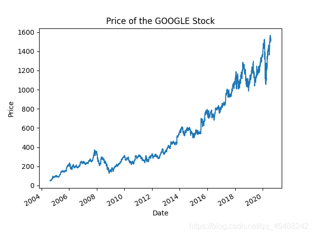
接下來就我們就將取其中的收盤價(擷取DataFrame物件的列會返回一個Series物件),呼叫Series物件的plot方法來繪圖

import numpy as np
import pandas as pd
import matplotlib.pyplot as plt
import  pandas_datareader.data as web
import yfinance as yf
import datetime
yf.pdr_override()


google=web.get_data_yahoo('GOOGL',start='2004-08-19',end='2020-07-31',data_source='google')
print(google.head())
print(type(google))
google['Close'].plot()
plt.xlabel('Date')
plt.ylabel('Price')
plt.title('Price of the GOOGLE Stock')
plt.show()
>>>
[*********************100%***********************]  1 of 1 completed
                 Open       High        Low      Close  Adj Close    Volume
Date                                                                       
2004-08-19  50.050049  52.082081  48.028027  50.220219  50.220219  44659000
2004-08-20  50.555557  54.594593  50.300301  54.209209  54.209209  22834300
2004-08-23  55.430431  56.796795  54.579578  54.754753  54.754753  18256100
2004-08-24  55.675674  55.855854  51.836838  52.487488  52.487488  15247300
2004-08-25  52.532532  54.054054  51.991993  53.053055  53.053055   9188600
<class 'pandas.core.frame.DataFrame'>

在这里插入图片描述

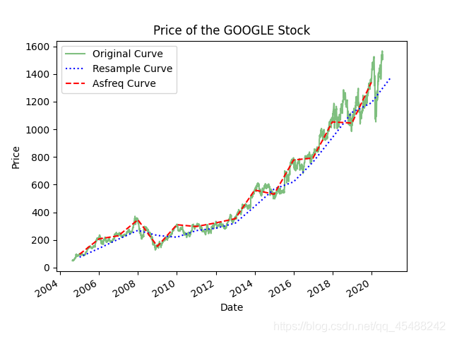
重新取樣與頻率轉換

我們在處理時間序列數據的時候,經常需要按照新的頻率來對數據進行重新取樣.例如上面我的Google股價是以天爲頻率的,我們如果想以月爲頻率的話,就需要每隔一個月進行重新取樣

對於重新取樣,我們可以呼叫resample()方法還活着asfreq()方法來完成,但是resample方法是以數據累計爲基礎,即我們對月進行重取樣的結果是一個月的所有值的和,我們需要手動求平均;而asfreq()方法則是以數據選擇爲基礎,即選取上個月的最後一個值

下面下麪我們將使用兩種方法對數據進行向後採樣(down-sample),這裏不是降採樣,而是向後採樣

google=pd.read_csv('GoogleStock.csv')
DatetimeIndex_1=pd.to_datetime(google['Date'])
google.index=DatetimeIndex_1
del google['Date']
google_close=google['Close']
google_close.plot(alpha=0.5,style='g-')
google_close.resample('BA').mean().plot(style='b:')
google_close.asfreq('BA').plot(style='r--')
plt.legend(['Original Curve','Resample Curve','Asfreq Curve'],loc='upper left')
plt.xlabel('Date')
plt.ylabel('Price')
plt.title('Price of the GOOGLE Stock')
plt.show()

在这里插入图片描述

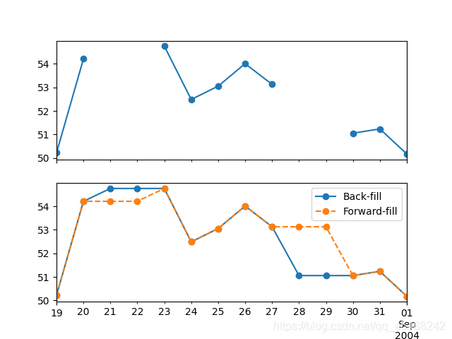
接下來我們再進行向前取樣(up-sample)由於向前取樣時會出現缺失值,所以asfreq()方法中有一個參數method來指定填充缺失值的方法

下面下麪我們對工作日數據按天進行重取樣,然後比較向前和向後填充,這裏我們用到了在matplotlib中將會講解的ax等內容.

google=pd.read_csv('GoogleStock.csv')
DatetimeIndex_1=pd.to_datetime(google['Date'])
google.index=DatetimeIndex_1
del google['Date']
google_close=google['Close']
fig, ax=plt.subplots(2,sharex=True)

data=google_close.iloc[:10]
data.asfreq('D').plot(ax=ax[0],marker='o')
data.asfreq('D',method='bfill').plot(ax=ax[1],style='-o')
data.asfreq('D',method='ffill').plot(ax=ax[1],style='--o')
ax[1].legend(['Back-fill','Forward-fill'])
plt.show()

在这里插入图片描述

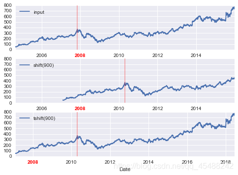
時間遷移

Pandas中另外一種常用的時間序列操作就是時間遷移,時間遷移指的就是將數據對應的時間進行改變

Pandas中有兩種解決時間遷移問題的方法:shift()和tshitf()方法

shift()方法是對數據進行遷移,而tshift是對索引進行遷移

google=pd.read_csv('GoogleStock.csv')
DatetimeIndex_1=pd.to_datetime(google['Date'])
google.index=DatetimeIndex_1
del google['Date']
google_close=google['Close']
fig, ax=plt.subplots(3,sharex=True)

google_close=google_close.asfreq('D',method='pad')                  #去除缺失值的影響

google_close.plot(ax=ax[0])
google_close.shift(900).plot(ax=ax[1])
google_close.shift(900).plot(ax=ax[2])

local_max=pd.to_datetime('2007-11-05')
offset=pd.Timedelta(900,'D')

ax[0].legend(['Original Curve'],loc=2)
ax[0].get_xticklabels()[4].set(weight='heavy',color='red')
ax[0].axvline(local_max,alpha=0.3,color='red')

ax[1].legend(['Shift(900)'],loc=2)
ax[1].get_xticklabels()[4].set(weight='heavy',color='red')
ax[1].axvline(local_max+offset,alpha=0.3,color='red')


ax[2].legend(['Tshift(900)'],loc=2)
ax[2].get_xticklabels()[1].set(weight='heavy',color='red')
ax[2].axvline(local_max+offset,alpha=0.3,color='red')

plt.show()

在这里插入图片描述

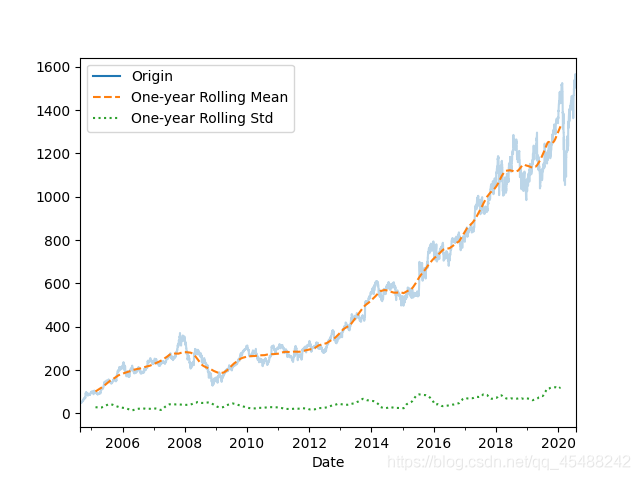
移動時間視窗

Pandas處理時間序列的第三種操作是移動統計值,計算移動統計值可以通過Series或者DataFrame物件的rolling()方法來實現

rolling()方法將會返回與groupby操作類似的結果

google=pd.read_csv('GoogleStock.csv')
DatetimeIndex_1=pd.to_datetime(google['Date'])
google.index=DatetimeIndex_1
del google['Date']
google_close=google['Close']

google_close=google_close.asfreq('D',method='pad')    

rolling=google_close.rolling(365,center=True)
data=pd.DataFrame({'Origin':google_close,'One-year Rolling Mean':rolling.mean(),'One-year Rolling Std':rolling.std()})
ax=data.plot(style=['-','--',':'])
ax.lines[0].set_alpha(0.3)
plt.show()

在这里插入图片描述

13.Pandas處理時間序列

文章目錄

Pandas處理時間序列

Python的日期與時間工具

原生Python的日期與時間工具:datetime與dateutil

建立日期

指定輸出

Numpy的日期與時間工具:datetime64型別

Numpy建立日期陣列

Numpy日期陣列的運算

Numpy的datetime64物件

datetime64物件的建立

datetime64物件的單位

Pandas的日期和時間工具

建立Timestamp物件

呼叫datetime和dateutil的方法

Pandas的時間序列:以時間作爲索引

建立時間序列索引

指定時間序列爲索引

Pandas的時間序列物件

to_datetime()函數

to_period()方法

date_range()函數

period_range()與timedelta_range()函數

Pandas時間頻率與偏移量

Pandas的重新取樣,遷移和視窗

獲取Google的股價數據

重新取樣與頻率轉換

時間遷移

移動時間視窗