【論文翻譯】Deep Residual Learning for Image Recognition

論文題目：Deep Residual Learning for Image Recognition
論文來源：IEEE CVPR(Conference on Computer Vision and Pattern Recognition)

Deep Residual Learning for Image Recognition

Kaiming He & Xiangyu Zhang & Shaoqing Ren & Jian Sun

Abstract

Deeper neural networks are more difficult to train. We present a residual learning framework to ease the training of networks that are substantially deeper than those used previously. We explicitly reformulate the layers as learning residual functions with reference to the layer inputs, instead of learning unreferenced functions. We provide comprehensive empirical evidence showing that these residual networks are easier to optimize,and can gain accuracy from considerably increased depth. On the ImageNet dataset we evaluate residualnets with adepth of up to152 layers—8× deeper than VGG nets but still having lower complexity.An ensemble of these residual nets achieves 3.57%error ontheImageNettestset. This result won the 1st place on the ILSVRC 2015 classification task. We also present analysis on CIFAR-10 with 100 and 1000 layers.

The depth of representations is of central importance for many visual recognition tasks. Solely due to our extremely deep representations, we obtain a 28% relative improvement on the COCO object detection dataset. Deep residual nets are foundations of our submissions to ILSVRC & COCO 2015 competitions, where we also won the 1st places on the tasks of ImageNet detection, ImageNet localization, COCO detection, and COCO segmentation.

摘要：更深的神經網路更難訓練，我們提出了一個殘差學習框架，以簡化比以前使用的網路更深的網路的訓練。我們明確地將層重述爲學習參考層輸入的殘差函數，而不是學習未參考的函數。我們提供了全面的經驗證據，表明這些殘差網路更容易優化，並且可以從大大增加的深度中獲得準確性。在ImageNet數據集上，我們評估了深度達152層的殘差網路，比VGG網路深8倍，但仍然具有較低的複雜性。這個結果贏得了ILSVRC 2015分類任務的第1名。我們還介紹了對CIFAR-10的100層和1000層的分析。表徵的深度對於許多視覺識別任務來說是至關重要的。僅僅由於我們極深的表徵，我們在COCO物件檢測數據集上獲得了28%的相對改進。深度殘差網是我們提交給ILSVRC & COCO 2015比賽的基礎，我們還在ImageNet檢測、ImageNet定位、COCO檢測和COCO分割等任務中獲得了第一名。

1.Introduction

Deep convolutional neural networks have led to a series of breakthroughs for image classification. Deep networks naturally integrate low/mid/highlevel features and classifiers in an end-to-end multilayer fashion, and the 「levels」 of features can be enriched by the number of stacked layers (depth).Recent evidence revealsthatnetworkdepthisofcrucialimportance, and the leading results on the challenging ImageNet dataset all exploit 「very deep」 models, with a depth of sixteen to thirty . Many other nontrivial visual recognition tasks have also greatly benefited from very deep models.

深度折積神經網路爲影象分類帶來了一系列的突破。深度網路自然地將從低、中、高層次的特徵和分類器以端到端多層的方式整合在一起，特徵的 "層次 "可以通過堆疊層數即深度來豐富。最近的證據表明，網路深度是至關重要的，在具有挑戰性的ImageNet數據集上的領先結果都利用了 "非常深度 "模型，深度爲16到30。許多其他非微不足道的視覺識別任務也從非常深的模型中獲益匪淺。

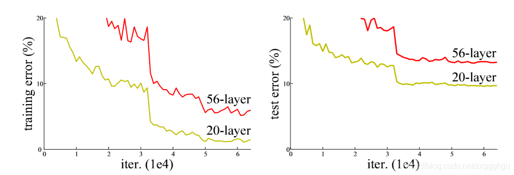
Figure 1. Training error (left) and test error (right) on CIFAR-10 with 20-layer and 56-layer 「plain」 networks. The deeper network has higher training error, and thus test error. Similar phenomena on ImageNet is presented in Fig. 4.

圖1. 20層和56層 "普通 "網路在CIFAR-10上的訓練誤差如左圖所示，測試誤差如右圖所示。較深的網路具有較高的訓練誤差，因此測試誤差也較高，類似的現象在ImageNet上呈現在圖4中。

Driven by the significance of depth, a question arises: Is learning better networks as easy as stacking more layers? An obstacle to answering this question was the notorious problem of vanishing/exploding gradients, which hamper convergence from the beginning. This problem, however, has been largely addressed by normalized initialization and intermediate normalization layers,which enable networks with tens of layers to start converging for stochastic gradient descent (SGD) with backpropagation.

When deeper networks are able to start converging, a degradation problem has been exposed: with the network depth increasing, accuracy gets saturated (which might be unsurprising) and then degrades rapidly. Unexpectedly, such degradation is not caused by overfitting, and adding more layers to a suitably deep model leads to higher training error,as reported in and thoroughly verified by our experiments. Fig. 1 shows a typical example.

The degradation (of training accuracy) indicates that not all systems are similarly easy to optimize. Let us consider a shallower architecture and its deeper counterpart that adds more layers onto it. There exists a solution by construction to the deeper model: the added layers are identity mapping, and the other layers are copied from the learned shallower model. The existence of this constructed solution indicates that a deeper model should produce no higher training error than its shallower counterpart. But experiments show that our current solvers on hand are unable to find solutions that are comparably good or better than the constructed solution (or unable to do so in feasible time).
在深度重要性的驅動下，一個問題出現了，學習更好的網路是否和堆疊更多的層數一樣容易？回答這個問題的一個障礙是臭名昭著的消失、爆炸梯度問題，它從一開始就阻礙了融合。然而，這個問題在很大程度上已經通過歸一化初始化和中間歸一化層得到了很大程度的解決，這使得有幾十層的網路能夠開始收斂，並進行隨機梯度下降和反向傳播。

當更深的網路能夠開始收斂時，一個退化的問題已經暴露出來，就是隨着網路深度的增加，精度變得飽和，這可能並不奇怪，然後迅速退化。出乎意料的是，這樣的退化並不是由過度建模造成的，而是由在一個適當深度的模型中，增加更多的層數會導致更高的訓練誤差，正如我們的實驗所報告並徹底驗證的那樣，圖1就是一個典型的例子。

訓練精度的下降表明，並不是所有的系統都同樣容易優化。讓我們考慮一個較淺的架構及其在其上增加更多層的較深的對應系統，深層模型存在一個通過構造的解決方案，即增加的層是身份對映，其他層是從學習的淺層模型中複製出來的。這種構造解的存在表明，一個較深的模型應該不會比它的較淺模型產生更高的訓練誤差。但實驗表明，我們目前手頭的求解器無法找到比較好或比構造解更好的解，或者無法在可行的時間內完成。

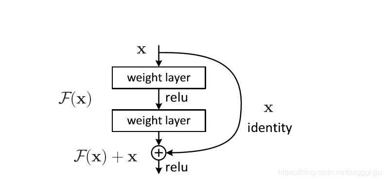
Figure 2. Residual learning: a building block.殘差學習構建

In this paper, we address the degradation problem by introducing a deep residual learning framework. Instead of hoping each few stacked layers directly fit a desired underlying mapping, we explicitly let these layers fit a residual mapping. Formally, denoting the desired underlying mapping as H(x), we let the stacked nonlinear layers fit another mapping of F(x) :=H(x)−x. The original mapping is recast into F(x)+x. We hypothesize that it is easier to optimize the residual mapping than to optimize the original, unreferenced mapping. To the extreme, if an identity mapping were optimal, it would be easier to push the residual to zero than to fit an identity mapping by a stack of nonlinear layers.

在本文中，我們通過引入一個深度殘差學習框架來解決退化問題。我們不希望每幾個堆疊層直接對應一個期望的底層對映，而是明確地讓這些層對應一個殘差對映。形式上，將期望的底層對映表示爲H(x)，我們讓堆疊的非線性層對應另一個對映F(x) :=H(x)-x。原始對映被重鑄爲F(x)+x。我們假設，優化殘差對映比優化原始的、未參照的對映更容易。極端地講，如果一個身份對映是最優的，那麼通過非線性層的堆疊，將殘差推到零比將身份對映對應更容易。

The formulation of F(x)+x can be realized by feedforward neural networks with 「shortcut connections」 (Fig. 2). Shortcut connections are those skipping one or more layers. In our case, the shortcut connections simply perform identity mapping, and their outputs are added to the outputs of the stacked layers (Fig. 2). Identity shortcut connections add neither extra parameter nor computational complexity. The entire network can still be trained end-to-end by SGD with backpropagation, and can be easily implemented using common libraries without modifying the solvers.

We present comprehensive experiments on ImageNet to show the degradation problem and evaluate our method. We show that: 1)Our extremely deep residual nets are easy to optimize, but the counterpart 「plain」 nets (that simply stack layers) exhibit higher training error when the depth increases; 2) Our deep residual nets can easily enjoy accuracy gains from greatly increased depth, producing results substantially better than previous networks.

Similar phenomena are also shown on the CIFAR-10 set , suggesting that the optimization difficulties and the effects of our method are not just akin to a particular dataset. We present successfully trained models on this dataset with over 100 layers, and explore models with over 1000 layers.

On the ImageNet classification dataset, we obtain excellent results by extremely deep residual nets. Our 152layer residual net is the deepest network ever presented on ImageNet, while still having lower complexity than VGG nets. Our ensemble has 3.57% top-5 error on the ImageNet test set, and won the 1st place in the ILSVRC 2015 classification competition. The extremely deep representations also have excellent generalization performance on other recognition tasks, and lead us to further win the 1st places on: ImageNet detection, ImageNet localization, COCO detection, and COCO segmentation in ILSVRC &COCO 2015 competitions. This strong evidence shows that the residual learning principle is generic,and we expect that it is applicable in other vision and non-vision problems.

F(x)+x的公式可以通過具有 "捷徑連線 "的前饋神經網路來實現，如圖2。捷徑連線是指那些跳過一層或多層的連線。在我們的案例中，捷徑連線只是執行身份對映，它們的輸出被新增到堆疊層的輸出中，如圖2所示。身份捷徑連線既沒有增加額外的參數，也沒有增加計算的複雜性。整個網路仍然可以通過SGD與反向傳播進行端到端訓練，並且可以在不修改求解器的情況下使用通用庫輕鬆實現。

我們介紹了在ImageNet上的綜合實驗，來顯示退化問題並評估我們的方法。我們得出： 1，我們的極深殘差網很容易優化，但對應的 "普通 "網，即那些只是簡單地堆疊層，在深度增加時表現出更高的訓練誤差；2，我們的深度殘差網可以很容易地享受到，由深度大幅增加帶來的精度提升，其產生的結果大大優於之前的網路。

類似的現象在CIFAR-10集上也有表現，說明我們方法的優化難度和效果並不只是類似於某一個特定的數據集。我們介紹了在這個數據集上成功訓練的超過100層的模型，並探索超過1000層的模型。

在ImageNet分類數據集上，我們通過極深的殘差網獲得了出色的結果。我們的152層殘差網是有史以來在ImageNet上呈現的最深的網路，同時其複雜度仍低於VGG網。我們的合集在ImageNet測試集上的前5個錯誤的錯誤率爲3.57％，並在ILSVRC 2015分類競賽中獲得第一名。極大的表現在其他識別任務上也有很好的泛化效能，並帶領我們進一步贏得了第1名。在ILSVRC &COCO 2015比賽中，ImageNet檢測、ImageNet定位、COCO檢測和COCO分割都獲得了第一名。這些有力的證據表明，殘差學習原理是通用的，我們期望它能適用於其他視覺和非視覺問題。

2.Related Work

Residual Representations. In image recognition, VLAD is a representation that encodes by the residual vectors with respect to a dictionary, and Fisher Vector can be formulated as a probabilistic version of VLAD. Both of them are powerful shallow representations for image retrieval and classification . For vector quantization, encoding residual vectors is shown to be more effective than encoding original vectors.

In low-level vision and computer graphics, for solving Partial Differential Equations (PDEs), the widely used Multigrid method reformulates the system as subproblems at multiple scales, where each subproblem is responsible for the residual solution between a coarser and a finer scale. An alternative to Multigrid is hierarchical basis preconditioning, which relies on variables that represent residual vectors between two scales. It has been shown that these solvers converge much faster than standard solvers that are unaware of the residual nature of the solutions. These methods suggest that a good reformulation or preconditioning can simplify the optimization.

殘差表示法:在影象識別中，VLAD是一種由殘差向量相對於字典進行編碼的表示方法，費舍爾向量可以被表述爲VLAD的概率版本,他們都是強大的淺層表示法，用於影象檢索和分類。對於向量量化，編碼殘差向量被證明比編碼原始向量更有效。

在低階視覺和計算機圖學中，爲了解決偏微分方程，廣泛使用的Multigrid方法將系統重構爲多個尺度的子問題，其中每個子問題負責一個較粗和一個較細尺度之間的殘差解。層次基礎預設是Multigrid的替代方法，它依賴於代表兩個尺度之間殘差向量的變數。已經證明，這些求解器的收斂速度比標準求解器快得多，因爲標準求解器不知道解的殘差性質。這些方法表明，一個好的重新計算或預設可以簡化優化。

Shortcut Connections. Practices and theories that lead to shortcut connections have been studied for a long time. An early practice of training multi-layer perceptrons (MLPs) is to add a linear layer connected from the network input to the output . In , a few intermediate layers are directly connected to auxiliary classifiers for addressing vanishing/exploding gradients. The papers of propose methods for centering layer responses, gradients, and propagated errors, implemented by shortcut connections. In , an 「inception」 layer is composed of a shortcut branch and a few deeper branches.

Concurrent with our work, 「highway networks」 present shortcut connections with gating functions. These gates are data-dependent and have parameters, in contrast to our identity shortcuts that are parameter-free. When a gated shortcut is 「closed」 (approaching zero), the layers in highway networks represent non-residual functions. On the contrary, our formulation always learns residual functions; our identity shortcuts are never closed, and all information is always passed through, with additional residual functions to be learned. In addition,highway networks have not demonstrated accuracy gains with extremely increased depth (e.g., over 100 layers).

捷徑連線：得到捷徑連線的實踐和理論已經研究了很長時間。在早期實踐中，訓練多層感知器是增加一個線性層，從網路輸入連線到輸出。在 幾個中間層直接連線到輔助分類器，用於解決消失、爆炸梯度。論文提出了通過快捷連線實現居中層響應，梯度和傳播錯誤的方法。其中一個 "起始 "層是由一個捷徑分支和幾個較深的分支組成。

與我們的工作同步，"高速公路網路 "呈現出具有門控功能的捷徑連線。這些門控函數是依賴於數據並有參數的，與我們的身份捷徑相反，它是無參數的。當一個門控捷徑被 "關閉"或快要關閉時，高速公路網路中的圖層就代表了非剩餘函數。相反，我們的公式總是學習殘差函數；我們的身份捷徑永遠不會被關閉，所有資訊總是被傳遞，還有額外的殘差函數需要學習。此外，高速公路網路並沒有顯示出隨着深度的極度增加而提高的精度。

3.Deep Residual Learning深度殘差學習

3.1.Residual Learning

Let us consider H(x) as an underlying mapping to be fit by a few stacked layers (not necessarily the entire net), with x denoting the inputs to the first of these layers. If one hypothesizes that multiple nonlinear layers can asymptotically approximate complicated functions, then it is equivalent to hypothesize that they can asymptotically approximate the residual functions, i.e., H(x)−x (assuming that the input and output are of the same dimensions). So rather than expect stacked layers to approximateH(x), we explicitly let these layers approximate a residual function F(x) :=H(x) − x. The original function thus becomes F(x)+x. Although both forms should be able to asymptotically approximate the desired functions (as hypothesized), the ease of learning might be different.

This reformulation is motivated by the counterintuitive phenomena about the degradation problem(Fig.1,left). As we discussed in the introduction, if the added layers can be constructed as identity mappings,a deeper model should have training error no greater than its shallower counterpart. The degradation problem suggests that the solvers might have difficulties in approximating identity mappings by multiple nonlinear layers. With the residual learning reformulation, if identity mappings are optimal, the solvers may simply drive the weights of the multiple nonlinear layers toward zero to approach identity mappings.

In real cases,it is unlikely that identity mappings are optimal, but our reformulation may help to precondition the problem. If the optimal function is closer to an identity mapping than to a zero mapping, it should be easier for the solver to find the perturbations with reference to an identity mapping, than to learn the function as a new one. We show by experiments (Fig.7) that the learned residual functionsin general have small responses, suggesting that identity mappings provide reasonable preconditioning.

讓我們把H(x)看作是由幾個堆疊層,不一定是整個網,構成的底層對映，x表示這些層的第幾層的輸入。如果假設多個非線性層可以漸進地逼近複雜函數，那麼就相當於假設它們可以漸進地逼近殘差函數，即H(x)-x,假設此時輸入和輸出的維度相同。因此，我們不期望堆疊層能夠近似H(x)，而是明確地讓這些堆疊層近似殘差函數F(x)=H(x)-x.因此，原始函數就變成了F(x)+x。雖然兩種形式都應該能夠漸進地逼近所需的函數，如假設的那樣，但學習的難易程度可能不同。

這種重構的目的是關於退化問題的反直覺現象，如圖1左圖。正如我們在前言中所討論的那樣，如果增加的層可以被構造爲身份對映，那麼一個較深的模型的訓練誤差應該不大於其較淺的模型。降級問題表明，求解者在通過多個非線性層來逼近身份對映時可能會有困難。通過殘差學習的重構，如果身份對映是最優的，求解器可能會簡單地將多個非線性層的權重趨近於零，以接近身份對映。

在實際情況下，身份對映不太可能是最優的，但我們的重構可能有助於爲問題提供前提條件。如果最優函數更接近於身份對映而不是零對映，那麼求解者參考身份對映來尋找幹擾應該比學習新的函數更容易。我們通過實驗，如圖7表明，學習到的殘差函數一般都有較小的響應，這說明身份對映提供了合理的預設。

3.2.Identity Mapping by Shortcuts

We adopt residual learning to every few stacked layers. A building block is shown in Fig. 2. Formally, in this paper we consider a building block defined as: y = F(x,{W_i})+x. (1) Here x and y are the input and output vectors of the layers considered. The function F(x,{Wi}) represents the residual mapping to be learned. For the example in Fig. 2 that has two layers, F = W₂σ(W₁x) in which σ denotes ReLU and the biases are omitted for simplifying notations. The operation F + x is performed by a shortcut connection and element-wise addition. We adopt the second nonlinearity after the addition (i.e., σ(y), see Fig. 2).

The shortcut connections in Eqn.(1)introduce neither extra parameter nor computation complexity. This is not only attractive in practice but also important in our comparisons between plain and residual networks. We can fairly compare plain/residual networks that simultaneously have the same number of parameters, depth, width, and computational cost (except for the negligible element-wise addition).

The dimensions of x and F must be equal in Eqn.(1). If this is not the case (e.g., when changing the input/output channels), we can perform a linear projection Ws by the shortcut connections to match the dimensions:y = F(x,{W_i})+W_sx. (2)
We can also use a square matrix W_s inEqn.(1). Butwewill show by experiments that the identity mapping is sufficient for addressing the degradation problem and is economical, and thus Ws is only used when matching dimensions.

The form of the residual function F is flexible. Experiments in this paper involve a function F that has two or three layers (Fig. 5), while more layers are possible. But if F has only a single layer,Eqn.(1)is similar to a linear layer: y = W₁x+x,for which we have not observed advantages. We also note that although the above notations are about fully-connected layers for simplicity, they are applicable to convolutional layers. The function F(x,{W_i}) can represent multiple convolutional layers. The element-wise addition is performed on two feature maps, channel by channel.

我們對每幾個堆疊層採用殘差學習。一個構件如圖2所示。形式上，在本文中，我們考慮一個構件的定義爲：y = F(x,{W_i})+x. 這裏x和y是所考慮的層的輸入和輸出向量。函數F(x,{Wi})表示要學習的殘差對映。對於圖2中具有兩層的例子，F = W₂σ(W₁x)，其中σ表示ReLU，爲了簡化符號，省略了偏置。F+x的操作是通過捷徑連線和元素相加來完成的。我們採用加法後的第二種非線性，即σ(y)，見圖2。

Eqn.(1)中的快捷連線既不引入額外的參數，也不增加計算的複雜性。這不僅在實踐中很有吸引力，而且在我們比較普通網路和殘差網路時也很重要。我們可以公平地比較樸素、殘差網路，它們同時具有相同的參數數、深度、寬度和計算成本，除了可忽略不計的元素加法。

在Eqn.(1)中，x和F的維度必須相等。如果不是這種情況，如改變輸入、輸出通道時，我們可以通過快捷連線進行線性投影Ws來匹配:y = F(x,{W_i})+W_sx. (2) 。我們也可以在Eqn.(1)中使用方陣W_s。但我們將通過實驗表明，身份對映對於解決退化問題是足夠的，而且是經濟的，因此W_s只在匹配維度時使用。

殘差函數F的形式是可延伸的。本文實驗涉及的函數F有兩層或三層，而更多的層數也是可能的。但如果F只有單層，則Eqn.(1)類似於線性層：y=W₁x+x，對此我們沒有觀察到優勢。我們還注意到，雖然爲了簡單起見，上面的符號是關於全連線層的，但它們適用於折積層。函數F(x,{W_i})可以表示多個折積層。元素加法是在兩個特徵圖上逐個通道進行的。

3.3.Network Architectures

We have tested various plain/residual nets, and have observed consistent phenomena. To provide instances for discussion, we describe two models for ImageNet as follows.
我們已經測試了各種普通、殘網，並觀察到了一致的現象。爲了提供討論的範例，我們將ImageNet的兩種模型描述如下`:

Plain Network. Our plain baselines (Fig. 3, middle) are mainly inspired by the philosophy of VGG nets. The convolutional layers mostly have 3×3 filters and follow two simple design rules: (i) for the same output feature map size, the layers have the same number of filters; and (ii) if the feature map size is halved, the number of filters is doubled so as to preserve the time complexity per layer. We perform downsampling directly by convolutional layers that have a stride of 2. The network ends with a global average pooling layer and a 1000-way fully-connected layer with softmax. The total number of weighted layers is 34 in Fig. 3 (middle).

It is worth noticing that our model has fewer filters and lower complexity than VGGnets(Fig.3,left). Our 34layer baseline has 3.6 billion FLOPs(multiply-adds),which is only 18% of VGG-19 (19.6 billion FLOPs).

我們的樸素基線（圖3，中間）主要受VGG網的理念啓發。折積層大多有3×3個過濾器，遵循兩個簡單的設計規則。(i)對於相同的輸出特徵圖大小，各層具有相同數量的過濾器；(ii)如果特徵圖大小減半，則filters的數量增加一倍，以保持每層的時間複雜度。我們直接通過折積層進行降採樣，折積層的步長爲2，網路的最後是一個全域性平均池化層和一個帶有softmax的1000路全連線層，圖3中，加權層總數爲34層。

值得注意的是，我們的模型比VGG網有更少的濾波器和更低的複雜度，如圖3左圖。我們的34層基線有36億個FLOPs，而VGG-19有196億個FLOPs，只佔VGG-19的18%。

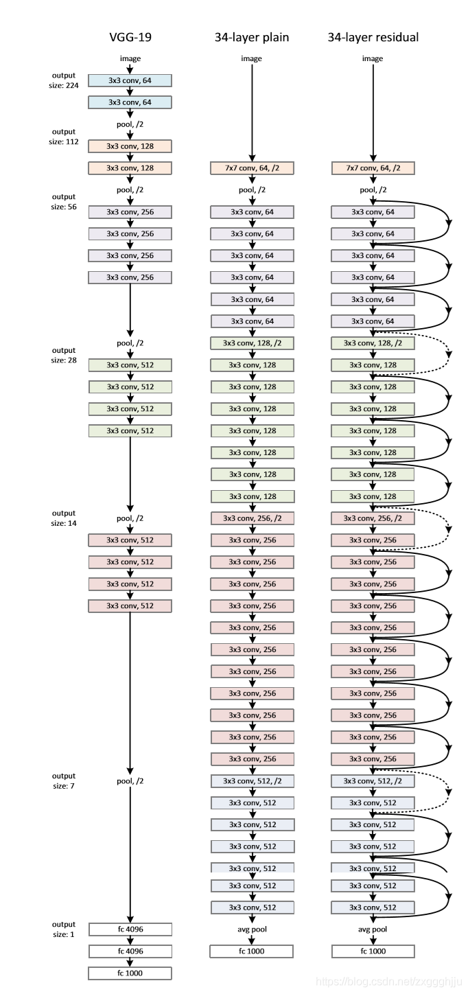
Figure 3. Example network architectures for ImageNet.
Left: the VGG-19 model (19.6 billion FLOPs) as a reference.
Middle: aplainnetworkwith34parameterlayers(3.6billionFLOPs).
Right: a residual network with 34 parameter layers (3.6 billion FLOPs). The dotted shortcuts increase dimensions.
Table 1 shows more details and other variants.

圖3. ImageNet的網路架構範例：
左：以VGG-19模型，其具有196億FLOPs爲參考
中間：具有34個參數層的普通網，其具有36億FLOPs
右：具有34個參數層的殘差網路，其具有36億FLOPs。虛線加劇增加了維度。
表1顯示了更多細節和其他變體。

Residual Network. Based on the above plain network, we insert shortcut connections (Fig. 3, right) which turn the network into its counterpart residual version. The identity shortcuts (Eqn.(1)) can be directly used when the input and output are of the same dimensions (solid line shortcuts in Fig.3). When the dimensions increase (dotted line shortcuts in Fig. 3), we consider two options: (A) The shortcut still performs identity mapping, with extra zero entries padded for increasing dimensions. This option introduces no extra parameter; (B) The projection shortcut in Eqn.(2) is used to match dimensions (done by 1×1 convolutions). For both options, when the shortcuts go across feature maps of two sizes, they are performed with a stride of 2.

在上述樸素網路的基礎上，我們插入快捷連線（圖3，右），將網路變成其對應的殘差版本。當輸入和輸出的維度相同時（圖3中的實線捷徑），可以直接使用身份捷徑（Eqn.(1)）。當維度增加時（圖3中的虛線捷徑），我們考慮兩種方案。(A)快捷方式仍然執行身份對映，尺寸增加時，額外的零條目填充。這個選項沒有引入額外的參數；（B）採用Eqn.（2）中的投影快捷方式進行維度匹配（由1×1折積完成）。對於這兩個選項，當捷徑橫跨兩種尺寸的特徵圖時，它們的步幅都是2。

3.4.Implementation

Our implementation for ImageNet follows the practice in [21, 40]. The image is resized with its shorter side randomly sampled in [256,480] for scale augmentation [40]. A 224×224 crop is randomly sampled from an image or its horizontal flip,with the per-pixel mean subtracted[21]. The standard color augmentation in[21]is used. We adopt batch normalization (BN) [16] right after each convolution and before activation, following [16]. We initialize the weights as in [12] and train all plain/residual nets from scratch. We use SGD with a mini-batch size of 256. The learning rate starts from 0.1 and is divided by 10 when the error plateaus, and the models are trained for up to 60×104 iterations. We use a weight decay of 0.0001 and a momentum of 0.9. We do not use dropout [13], following the practice in [16]. In testing, for comparison studies we adopt the standard 10-crop testing [21]. For best results, we adopt the fullyconvolutional form as in [40, 12], and average the scores at multiple scales (images are resized such that the shorter side is in{224,256,384,480,640}).

我們對ImageNet的實現沿用了[21，40]的做法。影象被調整大小，其較短的一面在[256,480]中隨機採樣，以進行比例增強[40]。從影象或其水平方向上隨機取樣224×224的裁剪，並減去每畫素的平均值[21]。採用[21]中的標準顏色增強法。我們在每次折積後和啓用前採用批次歸一化(batch normalization)[16],遵循[16]。我們按照[12]中的方法初始化權重，並從頭開始訓練所有普通/殘差網。我們使用SGD，迷你批次大小爲256。學習率從0.1開始，當誤差趨於平緩時除以10，模型的訓練次數最多爲60×104次迭代。我們使用0.0001的權重衰減和0.9的動量。我們沒有使用輟學[13]，沿用了[16]中的做法。在測試中，對於對比研究，我們採用標準的10-crop測試[21]。爲了獲得最佳結果，我們採用[40，12]中的全折積形式，並對多個尺度的分數進行平均（影象被調整大小，使短邊在{224,256,384,480,640}）。

4.Experiments

4.1.ImageNet Classification

We evaluate our method on the ImageNet 2012 classificationd ataset [35] that consists of 1000 classes. The models are trained on the 1.28 million training images, and evaluated on the 50k validation images. We also obtain a final result on the 100k test images, reported by the test server. We evaluate both top-1 and top-5 error rates.
Plain Networks. We first evaluate 18-layer and 34-layer plain nets. The 34-layer plain net is in Fig. 3 (middle). The 18-layer plain net is of a similar form. See Table 1 for detailed architectures.

我們在ImageNet 2012 的分類集上評估我們的方法，該分類集由1000個類組成。模型在128萬張訓練影象上進行訓練，並在50k張驗證影象上進行評估。我們還在10萬張測試影象上獲得了最終結果，由測試伺服器報告。我們評估了top-1和top-5的錯誤率。
Plain Networks。我們首先評估18層和34層的Plain Networks。34層的Plain Networks在圖3（中間）。18層的Plain Networks也是類似的形式。詳細架構見表1。

The results inTable 2 show that the deeper 34-layer plain net has higher validation error than the shallower 18-layer plain net. To reveal the reasons, in Fig. 4 (left) we compare their training/validation errors during the training procedure. We have observed the degradation problem the 34-layer plain net has higher training error throughout the whole training procedure, even though the solution space of the 18-layer plain network is a subspace of that of the 34-layer one.
表2中的結果顯示，較深的34層比較淺的18層有更高的驗證誤差。爲了揭示原因，在圖4（左）中，我們比較了它們在訓練過程中的訓練、驗證誤差。我們觀察到退化問題34層在整個訓練過程中具有較高的訓練誤差，儘管18層的解空間是34層的一個子空間。

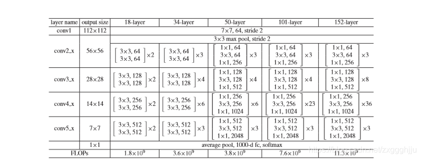
Table 1. Architectures for ImageNet. Building blocks are shown in brackets (see also Fig. 5), with the numbers of blocks stacked. Downsampling is performed by conv3_1, conv4_1, and conv5_1 with a stride of 2.
表1.ImageNet的架構。括號中顯示了構建塊（另請參見圖5）和模組堆疊的數量。 下採樣由conv3_1，conv4_1和conv5_1執行，步幅爲2。

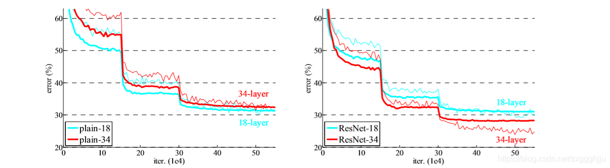
Figure 4. Training on ImageNet. Thin curves denote training error, and bold curves denote validation error of the center crops. Left: plain networks of 18 and 34 layers. Right: ResNets of 18 and 34 layers. In this plot, the residual networks have no extra parameter compared to their plain counterparts.
細曲線表示訓練誤差，粗曲線表示中心作物的驗證誤差。左：18層和34層的plain networks。右圖：18層和34層的plain networks。18層和34層的ResNets 在這個圖中，殘差網路與它們的plain networks相比沒有額外的參數。

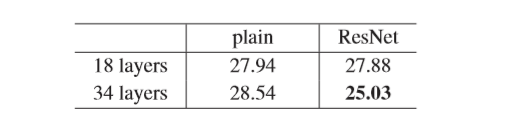
Table 2. Top-1 error (%, 10-crop testing) on ImageNet validation. Here the ResNets have no extra parameter compared to their plain counterparts. Fig. 4 shows the training procedures.
表2.在ImageNet驗證上的Top-1誤差。這裏的ResNets與它們的普通對應物相比沒有額外的參數。圖4顯示了訓練程式。

We argue that this optimization difficulty is unlikely to be caused by vanishing gradients. These plain networks are trained with BN [16], which ensures forward propagated signals to have non-zero variances. We also verify that the backward propagated gradients exhibit healthy norms with BN. So neither forward nor backward signals vanish. In fact, the 34-layer plain net is still able to achieve competitive accuracy (Table 3), suggesting that the solver works to some extent. We conjecture that the deep plain nets may have exponentially low convergence rates,which impact the reducing of the training error. The reason for such optimization difficulties will be studied in the future.

我們認爲，這種優化困難不太可能是由消失梯度引起的。這些 plain networks是用BN訓練的，它確保了前向傳播的信號具有非零變異。我們也用BN驗證了後向傳播的梯度表現出健康的規範。所以前向和後向信號都不會消失。事實上，34層的plain networks仍然能夠達到競爭性的精度（表3），說明解算器在一定程度上是有效的。我們推測，深層plain net可能具有指數級的低收斂率，這影響了訓練誤差的減小。這種優化困難的原因將在未來進行研究。

Residual Networks. Next we evaluate 18-layer and 34-layer residual nets (ResNets). The baseline architectures are the same as the above plain nets, expect that a shortcut connection is added to each pair of 3×3 filters as in Fig. 3 (right). In the first comparison (Table 2 and Fig. 4 right), we use identity mapping for all shortcuts and zero-padding for increasing dimensions (optionA).So they have no extra parameter compared to the plain counterparts. We have three major observations from Table 2 and Fig. 4. First, the situation is reversed with residual learning–the 34-layer ResNet is better than the18-layer ResNet (by 2.8%). More importantly, the 34-layer ResNet exhibits considerably lower training error and is generalizable to the validation data. This indicates that the degradation problem is well addressed in this setting and we manage to obtain accuracy gains from increased depth.

殘差網路。接下來我們評估18層和34層殘網路。基線架構與上述plain net相同，期望在每一對3×3 過濾中增加一個快捷連線，如圖3（右）。在第一個比較中，即表2和圖4右，我們對所有的捷徑使用身份對映，對增加的維度使用零填充.因此，與普通對應物相比，它們沒有額外的參數。從表2和圖4中我們有三個主要的觀察。首先，殘差學習的情況是相反的，34層的ResNet比18層的ResNet好2.8%。更重要的是，34層ResNet表現出相當低的訓練誤差，並且對驗證數據具有通用性。這說明在這種環境下，退化問題得到了很好的解決，我們設法通過增加深度來獲得精度的提升。

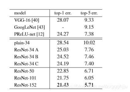
Table 3. Error rates (%, 10-crop testing) on ImageNet validation. VGG-16 is based on our test. ResNet-50/101/152 are of option B that only uses projections for increasing dimensions.
ImageNet驗證的錯誤率。VGG-16是基於我們的測試。ResNet-50/101/152屬於選項B，只使用投影來增加維度。

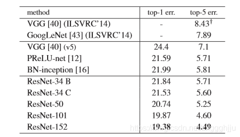
Table 4. Error rates (%) of single-model results on the ImageNet validation set (except reported on the test set).
ImageNet驗證集上單一模型結果的錯誤率,測試集上報告的除外。

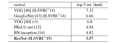
Table 5. Error rates (%) of ensembles. The top-5 error is on the test set of ImageNet and reported by the test server.
全部的錯誤率（%）。前5名的錯誤是在ImageNet的測試集上，由測試伺服器報告。

Second, compared to its plain counterpart, the 34-layer ResNet reduces the top-1 error by 3.5% (Table 2), resulting from the successfully reduced training error (Fig.4 right vs. left). This comparison verifies the effectiveness of residual learning on extremely deep systems.
Last, we also note that the 18-layer plain/residual nets are comparably accurate (Table 2), but the 18-layer ResNet converges faster (Fig. 4 right vs. left). When the net is 「not overly deep」(18 layers here),the current SGD solverisstill able to find good solutions to the plain net. In this case, the ResNet eases the optimization by providing faster convergence at the early stage.

其次，與它的普通對應物相比，34層ResNet減少了3.5%的top-1誤差（表2），這是由成功減少的訓練誤差造成的（Fig.4rightvs.left）。這個比較驗證了殘差學習在極深系統上的有效性。
最後，我們還注意到，18層的平網/殘網比較準確（見表2），但18層的ResNet收斂速度更快（圖4右與左對比課件）。當網 「不是太深」(這裏是18層)時，當前的SGD求解器仍然能夠找到 plain net的良好解。在這種情況下，ResNet通過在早期階段提供更快的收斂速度來緩解優化。

Identity vs. Projection Shortcuts. We have shown that parameter-free, identity shortcuts help with training. Next we investigate projection shortcuts(Eqn.(2)). InTable 3 we compare three options: (A)zero-padding shortcuts are used for increasing dimensions, and all shortcuts are parameterfree (the same as Table 2 and Fig. 4 right); (B) projection shortcuts are used for increasing dimensions,andother shortcuts are identity; and © all shortcuts are projections.
身份與投影捷徑，我們已經證明了無參數、身份的快捷方式有助於訓練。接下來我們研究投影快捷方式。在表3中，我們比較了三種方案。(A)零填充捷徑用於增加維度，所有的捷徑都是無參數的(與表2和圖4右相同)；(B)投影捷徑用於增加維度，其他捷徑都是身份捷徑；©所有的捷徑都是投影。

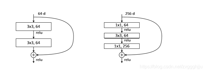
Figure 5. A deeper residual function F for ImageNet. Left: a building block (on 56×56 feature maps) as in Fig. 3 for ResNet34. Right: a 「bottleneck」 building block for ResNet-50/101/152.

圖5. ImageNet的更深層次的殘差函數F。左：ResNet34的一個構建塊（在56×56特徵圖上），如圖3。右：ResNet-50/101/152的一個 "瓶頸 "構建塊`。

Table 3 shows that all three options are considerably better than the plain counterpart. B is slightly better thanA.We argue that this is because the zero-padded dimensions in A indeed have no residual learning. C is marginally betterthan B, and we attribute this to the extra parameters introduced by many (thirteen) projection shortcuts. But the small differences among A/B/C indicate that projection shortcuts are not essential for addressing the degradation problem. So we do not use option C in the rest of this paper,to reduce memory/time complexity and model sizes. Identity shortcuts are particularly important for not increasing the complexity of the bottleneck architectures that are introduced below.

表3顯示，三個選項都比普通對應的選項好很多。B比A.我們認爲，這是因爲A中的零填充維度確實沒有殘餘學習。C略好於B，我們認爲這是由於許多（十三種）投影快捷方式引入的額外參數。但是A、B、C之間的差異很小，這說明投影快捷鍵對於解決退化問題並不是必不可少的。所以我們在本文其餘部分沒有使用選項C,以降低記憶體/時間的複雜性和模型大小。身份捷徑對於不增加下面 下麪介紹的瓶頸架構的複雜性尤爲重要。

Deeper Bottleneck Architectures. Next we describe our deeper nets for ImageNet. Because of concerns on the training time that we can afford, we modify the building block as a bottleneck design⁴. For each residual function F, we use a stack of 3 layers instead of 2(Fig.5). The three layers are1×1,3×3,and1×1 convolutions,where the 1×1 layers are responsible for reducing and then increasing (restoring) dimensions,leaving the 3×3 layer a bottleneck with smaller input/output dimensions. Fig. 5 shows an example, where both designs have similar time complexity.

The parameter-free identity shortcuts are particularly important for the bottleneck architectures. If the identity shortcut in Fig. 5 (right) is replaced with projection, one can show that the time complexity and model size are doubled, as the shortcut is connected to the two high-dimensional ends. So identity shortcuts lead to more efficient models for the bottleneck designs.

更深層次的瓶頸架構。接下來我們描述一下我們的ImageNet的深度網。由於擔心我們能承受的訓練時間，我們修改了構件作爲瓶頸設計。對於每個殘差函數F，我們使用一個3層的堆疊代替2層(見圖5)。這三層分別是1×1,3×3,和1×1折積，其中1×1層負責減少然後增加(恢復)維度，留下3×3層是一個輸入、輸出維度較小的瓶頸。圖5是一個例子，兩種設計的時間複雜度相似。
無參數的身份捷徑對於瓶頸架構尤爲重要。如果將圖5（右）中的身份捷徑替換爲投影，可以看出時間複雜度和模型尺寸都增加了一倍，因爲捷徑連線到兩個高維端。所以，身份捷徑可以使瓶頸設計的模型更加有效。

50-layer ResNet: We replace each 2-layer block in the 34-layer net with this 3-layer bottleneck block, resulting in a 50-layer ResNet (Table1). We use option B for increasing dimensions. This model has 3.8 billion FLOPs.

101-layer and 152-layer ResNets: We construct 101layer and 152-layer ResNets by using more 3-layer blocks (Table 1). Remarkably, although the depth is significantly increased, the 152-layer ResNet (11.3 billion FLOPs) still has lower complexity than VGG-16/19 nets (15.3/19.6 billion FLOPs).

The 50/101/152-layer ResNets are more accurate than the 34-layer ones by considerable margins (Table 3 and 4). We do not observe the degradation problem and thus enjoy significant accuracy gains from considerably increased depth. The benefits of depth are witnessed for all evaluation metrics (Table 3 and 4).

50層ResNet 我們用這個3層瓶頸塊替換34層網中的每個2層塊，從而得到一個50層的ResNet（見表1）。我們使用選項B來增加維度。這個模型有38億個FLOPs。

101層和152層的 ResNets 我們通過使用更多的3層塊來構建101層和152層ResNets（見表1）。值得注意的是，雖然深度明顯增加，但152層ResNet，其含113億FLOPs的複雜度仍然低於VGG-16/19網，其含153或196億FLOPs。

50、101、152層的ResNets比34層的ResNets要精確得多（見表3和4）。我們沒有觀察到退化問題，因此享受到大幅增加的深度所帶來的明顯的精度提升。所有的評估指標都可以看到深度的好處（見表3和4）。

Comparisons with State-of-the-art Methods. In Table 4 we compare with the previous best single-model results. Our baseline 34-layer ResNets have achieved very competitive accuracy. Our 152-layer ResNet has a single-model top-5 validation error of 4.49%. This single-model result outperforms all previous ensemble results (Table 5). We combine six models of different depth to form an ensemble (only with two 152-layer ones at the time of submitting). This leads to 3.57% top-5 error on the test set (Table 5). This entry won the 1st place in ILSVRC 2015.

對比最先進方法，在表4中，我們與之前最好的單模型結果進行了比較。我們的基線34層ResNets已經達到了非常有競爭力的精度。我們的152層ResNet的單模型前5名驗證誤差爲4.49%。這個單模型結果優於之前所有的合集結果（表5）。我們將6個不同深度的模型組合起來形成一個合集（提交時只有兩個152層的）。這導致測試集上前5名的誤差爲3.57%（表5）。該作品獲得了2015年ILSVRC的第一名。

4.2.CIFAR-10 and Analysis

We conducted more studies on the CIFAR-10 dataset [20], which consists of 50k training images and 10k testing images in 10 classes. We present experiments trained on the training set and evaluated on the test set. Our focus is on the behaviors of extremely deep networks, but not on pushing the state-of-the-art results, so we intentionally use simple architectures as follows.

我們對CIFAR-10數據集[20]進行了更多的研究，該數據集由10類50k張訓練影象和10k張測試影象組成。我們介紹了在訓練集上訓練的實驗和在測試集上評估的實驗。我們的重點是極深網路的行爲，但不是推崇最先進的結果，所以我們有意使用簡單的架構，如下所示。

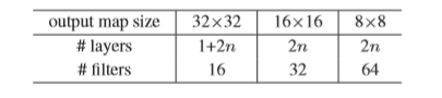
The plain/residual architectures follow the form in Fig.3 (middle/right). The network inputs are 32×32 images,with the per-pixel mean subtracted. The first layeris 3×3 convolutions. Then we use a stack of 6n layers with 3×3 convolutions on the feature maps of sizes{32,16,8} respectively, with 2n layers for each feature map size. The numbers of filtersare{16,32,64}respectively. The subsampling is performed by convolutions with astride of 2. The network ends with a global average pooling, a 10-way fully-connected layer,and softmax. There are totally 6n+2 stacked weighted layers. The following table summarizes the architecture:

普通、殘差架構的形式如圖3中、右。網路輸入爲32×32的影象，並減去每個畫素的平均值。第五層是3×3的折積。然後我們在尺寸爲{32,16,8}的特徵圖上分別用3×3折積堆疊6n層，每個特徵圖尺寸爲2n層。過濾器的數量分別爲{16,32,64}。通過跨度爲2的折積進行二次採樣。網路以全域性平均池，10路全連線層和softmax結尾. 共有6n+2個堆疊加權層。下表總結了架構：

When shortcut connections are used, they are connected to the pairs of 3×3 layers (totally 3n shortcuts). On this dataset we use identity shortcuts in all cases(i.e.,optionA),so our residual models have exactly the same depth, width, and number of parameters as the plain counterparts.

當使用快捷鍵連線時，它們被連線到3×3層的對子上，共3n個快捷鍵。在這個數據集上，我們在所有情況下都使用了身份快捷鍵，即選項A，所以我們的殘差模型的深度、寬度和參數數量與普通對應模型完全相同。

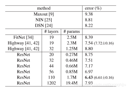
Table 6. Classification error on the CIFAR-10 test set. All methods are with data augmentation. ForResNet-110,we run it 5times and show 「best (mean±std)」 as in [42].
表6.CIFAR-10測試集的分類誤差 。所有方法都有數據增強。對於ResNet-110,我們執行了5次,並顯示 「最佳(平均值±std)」,如[42]。

We use a weight decay of 0.0001 and momentum of 0.9, and adopt the weight initialization in [12] and BN [16] but with no dropout. These models are trained with a minibatch size of 128 on two GPUs. We start with a learning rate of 0.1, divide it by 10 at 32k and 48k iterations, and terminate training at 64k iterations, which is determined on a 45k/5k train/val split. We follow the simple data augmentation in [24] for training: 4 pixels are padded on each side, and a 32×32 crop is randomly sampled from the padded image or its horizontal flip. For testing, we only evaluate the single view of the original 32×32 image.

We compare n = {3,5,7,9}, leading to 20, 32, 44, and 56-layer networks. Fig. 6 (left) shows the behaviors of the plain nets. The deep plain nets suffer from increased depth, and exhibit higher training error when going deeper. This phenomenon is similar to that on ImageNet (Fig.4,left) and on MNIST (see [41]), suggesting that such an optimization difficulty is a fundamental problem.

Fig. 6 (middle) shows the behaviors of ResNets. Also similar to the ImageNet cases (Fig. 4, right), our ResNets manage to overcome the optimization difficulty and demonstrate accuracy gains when the depth increases.

We further explore n = 18 that leads to a 110-layer ResNet. In this case, we find that the initial learning rate of 0.1 is slightly too large to start converging⁵So we use 0.01 to warm up the training until the training error is below 80%(about 400 iterations ), and then go back to 0.1and continue training. The rest of the learning schedule is as done previously. This 110-layer network converges well (Fig. 6, middle). It has fewer parameters than other deep and thin networks such as FitNet [34] and Highway [41] (Table 6), yet is among the state-of-the-art results (6.43%, Table 6).

我們使用0.0001的權重衰減和0.9的動量，並採用[12]和BN[16]中的權重初始化，但沒有dropout。這些模型在兩個GPU上以128個最小批次大小進行訓練。我們從0.1的學習率開始，在32k和48k迭代時將其除以10，並在64k迭代時終止訓練，這是在45k或5k的訓練或值分割上確定的。我們按照[24]中的簡單數據擴增進行訓練：每邊墊上4個畫素，從墊上的影象或其水平fl中隨機抽取一個32×32的裁剪。對於測試，我們只評估原始32×32影象的單檢視。

我們比較n = {3,5,7,9}，得出20、32、44和56層網路。 圖6（左）顯示了普通網路的行爲。 深層普通網受到深度增加的影響，當深入時表現出更高的訓練錯誤。 這種現象類似於ImageNet（圖4，左）和MNIST（參見[41]）上的現象，表明這種優化困難是一個基本問題。

圖6（中間）顯示了ResNets的行爲。同樣類似於ImageNet案例（圖4，右），我們的ResNets設法克服了優化的困難，並在深度增加時表現出精度的提高。

我們進一步探索n = 18，得到了110層的ResNet。在這種情況下，我們發現0.1的初始學習率稍大，無法開始收斂。所以我們使用0.01來預熱訓練，直到訓練誤差低於80%(約400次迭代)，然後回到0.1並繼續訓練。其餘的學習計劃和之前一樣。這個110層的網路收斂性很好（圖6，中間）。它的參數比FitNet[34]和Highway[41]等其他深層和薄層網路少(見表6)，卻屬於最先進的結果(6.43%，表6)。

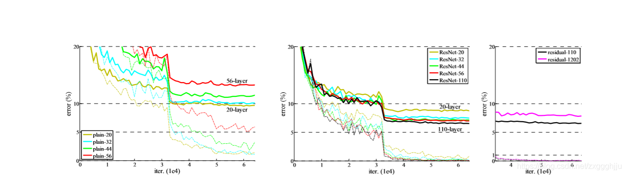
Figure 6. Training on CIFAR-10. Dashed lines denote training error, and bold lines denote testing error. Left: plain networks. The error of plain-110 is higher than 60% and not displayed. Middle: ResNets. Right: ResNets with 110 and 1202 layers.

圖6：在CIFAR-10上進行訓練。虛線表示訓練誤差，粗線表示測試誤差。左：plain network。plain-110的誤差高於60%，並且不顯示。中間：ResNets. 右圖：有110層和1202層的ResNets。

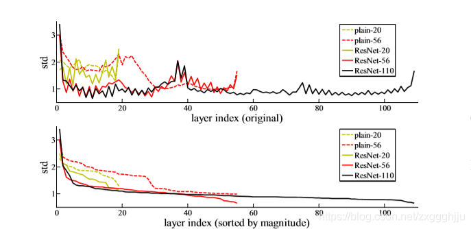
Figure 7. Standard deviations (std) of layer responses on CIFAR10. The responses are the outputs of each 3×3 layer, after BN and before nonlinearity. Top: the layers are shown in their original order. Bottom: the responses are ranked in descending order.

圖7.CIFAR10上各層響應的標準偏差（std）。這些響應是每個3×3層的輸出，在BN之後和非線性之前。頂部：各層以其原始順序顯示。底部：響應按降序排列。

Analysis of Layer Responses. Fig. 7 shows the standard deviations (std) of the layer responses. The responses are the outputs of each 3×3 layer, after BN and before other nonlinearity (ReLU/addition). For ResNets, this analysis reveals the response strength of the residual functions. Fig.7 shows that ResNets have generally smaller responses than their plain counterparts. These results support our basic motivation (Sec.3.1) that the residual functions might be generally closer to zero than the non-residual functions. We also notice that the deeper ResNet has smaller magnitudes of responses,as evidenced by the comparisons among ResNet-20, 56, and 110 in Fig. 7. When there are more layers, an individual layer of ResNets tends to modify the signal less.

層級響應分析：圖7顯示了各層響應的標準偏差（std）。這些響應是每個3×3層的輸出，在BN之後和其他非線性（ReLU或附加）之前。對於ResNets，這種分析揭示了殘差函數的響應強度。圖7顯示，ResNets的響應一般比它們的普通對應物小。這些結果支援了我們的基本動機（Sec.3.1），即殘差函數可能一般比非殘差函數更接近於零。我們還注意到，較深的ResNet具有較小的響應幅度，圖7中ResNet-20、56和110之間的比較就證明了這一點。當層數較多時，單個層的ResNet對信號的修改往往較小。

Exploring Over 1000 layers. We explore an aggressively deep model of over 1000 layers. We set n = 200 that leadstoa1202-layer network,which is trained as described above. Our method shows no optimization difficulty, and this 103-layer network is able to achieve training error <0.1% (Fig. 6, right). Its test error is still fairly good (7.93%, Table 6).

But there are still open problems on such aggressively deep models. The testing result of this 1202-layer network is worse than that of our 110-layer network, although both have similar training error. We argue that this is because of overfitting. The 1202-layer network may be unnecessarily large (19.4M) for this small dataset. Strong regularization such as maxout [9] or dropout [13] is applied to obtain the best results([9,25,24,34]) on this dataset. In this paper,we use no maxout/dropout and just simply impose regularization via deep and thin architectures by design, without distracting from the focus on the difficulties of optimization. But combining with stronger regularization may improve results, which we will study in the future.

探索超過1000層：我們探索了一個超過1000層的深度模型。我們設定n=200，導致了一個1202層的網路，訓練如上所述。我們的方法沒有顯示出優化的難度，這個103層的網路能夠實現訓練誤差<0.1%（圖6，右），其測試誤差還是相當不錯的（7.93%，表6）。

但是在這種激進的深度模型上仍然存在開放性的問題。這個1202層網路的測試結果比我們110層網路的測試結果要差，雖然兩者的訓練誤差相似。我們認爲，這是因爲過度定型。對於這個小數據集來說，1202層網路可能是不必要的大（19.4M）。使用強正則化，如maxout[9]或dropout[13]被應用於這個數據集上以獲得最佳結果([9,25,24,34])。在本文中,我們沒有使用maxout/dropout,只是簡單地通過深層和薄層架構的設計來施加正則化,而不分散對優化的關注點。但結合更強的正則化可能會改善結果，我們將在未來研究。

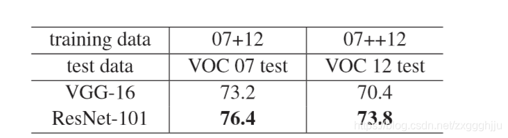
Table 7. Object detection mAP (%) on the PASCAL VOC 2007/2012 test sets using baseline Faster R-CNN. See also appendix for better results.
使用基準Faster R-CNN在PASCAL VOC 2007/2012測試集中進行的物件檢測mAP（％）。 另請參見附錄以獲得更好的結果。

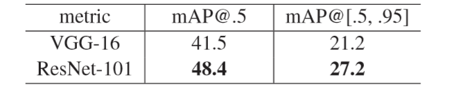
Table 8. Object detection mAP (%) on the COCO validation set using baseline Faster R-CNN.See also appendix for better results.
使用基線Faster R-CNN的COCO驗證集上的物件檢測mAP(%).另請參見附錄以獲得更好的結果。

4.3.Object Detection on PASCAL and MS COCO

PASCAL和MS COCO上的目標檢測

Our method has good generalization performance on other recognition tasks. Table 7 and 8 show the object detection baseline results on PASCAL VOC 2007 and 2012 [5] and COCO[26]. We adopt Faster R-CNN [32] as the detection method. Here we are interested in the improvements of replacing VGG-16 [40] with ResNet-101. The detection implementation (see appendix) of using both models is the same,so the gains can only be attributed to better networks. Most remarkably, on the challenging COCO dataset we obtaina 6.0% increase in COCO’s standard metric(mAP@[.5, .95]), which is a 28% relative improvement. This gain is solely due to the learned representations.

Based on deep residual nets, we won the 1st places in several tracks in ILSVRC & COCO 2015 competitions: ImageNet detection, ImageNet localization, COCO detection, and COCO segmentation. The details are in the appendix.

我們的方法在其他識別任務上具有良好的泛化效能。表7和表8是PASCAL VOC 2007和2012[5]以及COCO[26]上的物件檢測基線結果。我們採用Faster R-CNN[32]作爲檢測方法。這裏我們感興趣的是用ResNet-101替換VGG-16[40]的改進。使用這兩種模型的檢測實現(見附錄)都是一樣的，所以收益只能歸功於更好的網路。最值得注意的是，在具有挑戰性的COCO數據集上，我們獲得了COCO標準度量 6.0%的提升，相對提高了28%。這個增益完全歸功於學習的表示。

基於深度殘差網路，我們在ILSVRC & COCO 2015比賽中獲得了多個賽道的第一名。ImageNet檢測、ImageNet定位、COCO檢測和COCO分割。詳情見附錄。

========================================================================================================
References

[1] Y.Bengio,P.Simard,andP.Frasconi. Learninglong-termdependencies with gradient descent is difficult. IEEE Transactions on Neural Networks, 5(2):157–166, 1994.
[2] C. M. Bishop. Neural networks for pattern recognition. Oxford university press, 1995.
[3] W. L. Briggs, S. F. McCormick, et al. A Multigrid Tutorial. Siam, 2000.
[4] K. Chatfield, V. Lempitsky, A. Vedaldi, and A. Zisserman. The devil is in the details: an evaluation of recent feature encoding methods. In BMVC, 2011.
[5] M. Everingham, L. Van Gool, C. K. Williams, J. Winn, and A. Zisserman. The Pascal Visual Object Classes (VOC) Challenge. IJCV, pages 303–338, 2010.
[6] R. Girshick. Fast R-CNN. In ICCV, 2015.
[7] R. Girshick, J. Donahue, T. Darrell, and J. Malik. Rich feature hierarchies for accurate object detection and semantic segmentation. In CVPR, 2014.
[8] X. Glorot and Y. Bengio. Understanding the difficulty of training deep feedforward neural networks. In AISTATS, 2010.
[9] I. J. Goodfellow, D. Warde-Farley, M. Mirza, A. Courville, and Y. Bengio. Maxout networks. arXiv:1302.4389, 2013.
[10] K.HeandJ.Sun. Convolutionalneuralnetworksatconstrainedtime cost. In CVPR, 2015.
[11] K.He,X.Zhang,S.Ren,andJ.Sun. Spatialpyramidpoolingindeep convolutional networks for visual recognition. In ECCV, 2014.
[12] K. He, X. Zhang, S. Ren, and J. Sun. Delving deep into rectifiers: Surpassing human-level performance on imagenet classification. In ICCV, 2015.
[13] G. E. Hinton, N. Srivastava, A. Krizhevsky, I. Sutskever, and R. R. Salakhutdinov. Improving neural networks by preventing coadaptation of feature detectors. arXiv:1207.0580, 2012.
[14] S. Hochreiter. Untersuchungen zu dynamischen neuronalen netzen. Diploma thesis, TU Munich, 1991.
[15] S.HochreiterandJ.Schmidhuber. Longshort-termmemory. Neural computation, 9(8):1735–1780, 1997.
[16] S. Ioffe and C. Szegedy. Batch normalization: Accelerating deep networktrainingbyreducinginternalcovariateshift. InICML,2015.
[17] H.Jegou,M.Douze,andC.Schmid. Productquantizationfornearest neighbor search. TPAMI, 33, 2011.
[18] H. Jegou, F. Perronnin, M. Douze, J. Sanchez, P. Perez, and C.Schmid. Aggregatinglocalimagedescriptorsintocompactcodes. TPAMI, 2012.
[19] Y. Jia, E. Shelhamer, J. Donahue, S. Karayev, J. Long, R. Girshick, S.Guadarrama,andT.Darrell. Caffe: Convolutionalarchitecturefor fast feature embedding. arXiv:1408.5093, 2014.
[20] A. Krizhevsky. Learning multiple layers of features from tiny images. Tech Report, 2009.
[21] A. Krizhevsky, I. Sutskever, and G. Hinton. Imagenet classification with deep convolutional neural networks. In NIPS, 2012.
[22] Y. LeCun, B. Boser, J. S. Denker, D. Henderson, R. E. Howard, W. Hubbard, and L. D. Jackel. Backpropagation applied to handwritten zip code recognition. Neural computation, 1989.
[23] Y.LeCun,L.Bottou,G.B.Orr,andK.-R.M¨uller. Efficientbackprop. InNeuralNetworks: TricksoftheTrade,pages9–50.Springer,1998.
[24] C.-Y. Lee, S. Xie, P. Gallagher, Z. Zhang, and Z. Tu. Deeplysupervised nets. arXiv:1409.5185, 2014.
[25] M.Lin,Q.Chen,andS.Yan. Networkinnetwork. arXiv:1312.4400, 2013.
[26] T.-Y. Lin, M. Maire, S. Belongie, J. Hays, P. Perona, D. Ramanan, P. Doll´ar, and C. L. Zitnick. Microsoft COCO: Common objects in context. In ECCV. 2014.
[27] J. Long, E. Shelhamer, and T. Darrell. Fully convolutional networks for semantic segmentation. In CVPR, 2015.
[28] G. Mont´ufar, R. Pascanu, K. Cho, and Y. Bengio. On the number of linear regions of deep neural networks. In NIPS, 2014.
[29] V. Nair and G. E. Hinton. Rectified linear units improve restricted boltzmann machines. In ICML, 2010.
[30] F. Perronnin and C. Dance. Fisher kernels on visual vocabularies for image categorization. In CVPR, 2007.
[31] T. Raiko, H. Valpola, and Y. LeCun. Deep learning made easier by linear transformations in perceptrons. In AISTATS, 2012.
[32] S. Ren, K. He, R. Girshick, and J. Sun. Faster R-CNN: Towards real-time object detection with region proposal networks. In NIPS, 2015.
[33] B. D. Ripley. Pattern recognition and neural networks. Cambridge university press, 1996.
[34] A. Romero, N. Ballas, S. E. Kahou, A. Chassang, C. Gatta, and Y. Bengio. Fitnets: Hints for thin deep nets. In ICLR, 2015.
[35] O. Russakovsky, J. Deng, H. Su, J. Krause, S. Satheesh, S. Ma, Z. Huang, A. Karpathy, A. Khosla, M. Bernstein, et al. Imagenet large scale visual recognition challenge. arXiv:1409.0575, 2014.
[36] A. M. Saxe, J. L. McClelland, and S. Ganguli. Exact solutions to the nonlinear dynamics of learning in deep linear neural networks. arXiv:1312.6120, 2013.
[37] N.N.Schraudolph. Acceleratedgradientdescentbyfactor-centering decomposition. Technical report, 1998.
[38] N. N. Schraudolph. Centering neural network gradient factors. In Neural Networks: Tricks of the Trade, pages 207–226. Springer, 1998.
[39] P. Sermanet, D. Eigen, X. Zhang, M. Mathieu, R. Fergus, and Y. LeCun. Overfeat: Integrated recognition, localization and detection using convolutional networks. In ICLR, 2014.
[40] K. Simonyan and A. Zisserman. Very deep convolutional networks for large-scale image recognition. In ICLR, 2015.
[41] R. K. Srivastava, K. Greff, and J. Schmidhuber. Highway networks. arXiv:1505.00387, 2015.
[42] R. K. Srivastava, K. Greff, and J. Schmidhuber. Training very deep networks. 1507.06228, 2015.
[43] C.Szegedy,W.Liu,Y.Jia,P.Sermanet,S.Reed,D.Anguelov,D.Erhan, V. Vanhoucke, and A. Rabinovich. Going deeper with convolutions. In CVPR, 2015.
[44] R. Szeliski. Fast surface interpolation using hierarchical basis functions. TPAMI, 1990.
[45] R. Szeliski. Locally adapted hierarchical basis preconditioning. In SIGGRAPH, 2006.
[46] T. Vatanen, T. Raiko, H. Valpola, and Y. LeCun. Pushing stochastic gradient towards second-order methods–backpropagation learning with transformations in nonlinearities. In Neural Information Processing, 2013.
[47] A. Vedaldi and B. Fulkerson. VLFeat: An open and portable library of computer vision algorithms, 2008.
[48] W. Venables and B. Ripley. Modern applied statistics with s-plus. 1999.
[49] M. D. Zeiler and R. Fergus. Visualizing and understanding convolutional neural networks. In ECCV, 2014.